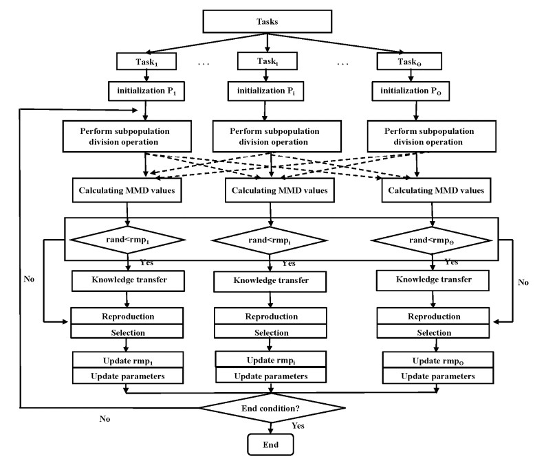
Evolutionary multitasking optimization (EMTO) handles multiple tasks simultaneously by transferring and sharing valuable knowledge from other relevant tasks. How to effectively identify transferred knowledge and reduce negative knowledge transfer are two key issues in EMTO. Many existing EMTO algorithms treat the elite solutions in tasks as transferred knowledge between tasks. However, these algorithms may not be effective enough when the global optimums of the tasks are far apart. In this paper, we study an adaptive evolutionary multitasking optimization algorithm based on population distribution information to find valuable transferred knowledge and weaken the negative transfer between tasks. In this paper, we first divide each task population into K sub-populations based on the fitness values of the individuals, and then the maximum mean discrepancy (MMD) is utilized to calculate the distribution difference between each sub-population in the source task and the sub-population where the best solution of the target task is located. Among the sub-populations of the source task, the sub-population with the smallest MMD value is selected, and the individuals in it are used as transferred individuals. In this way, the solution chosen for the transfer may be an elite solution or some other solution. In addition, an improved randomized interaction probability is also included in the proposed algorithm to adjust the intensity of inter-task interactions. The experimental results on two multitasking test suites demonstrate that the proposed algorithm achieves high solution accuracy and fast convergence for most problems, especially for problems with low relevance.
Citation: Xiaoyu Li, Lei Wang, Qiaoyong Jiang, Qingzheng Xu. An adaptive multitasking optimization algorithm based on population distribution[J]. Mathematical Biosciences and Engineering, 2024, 21(2): 2432-2457. doi: 10.3934/mbe.2024107
Evolutionary multitasking optimization (EMTO) handles multiple tasks simultaneously by transferring and sharing valuable knowledge from other relevant tasks. How to effectively identify transferred knowledge and reduce negative knowledge transfer are two key issues in EMTO. Many existing EMTO algorithms treat the elite solutions in tasks as transferred knowledge between tasks. However, these algorithms may not be effective enough when the global optimums of the tasks are far apart. In this paper, we study an adaptive evolutionary multitasking optimization algorithm based on population distribution information to find valuable transferred knowledge and weaken the negative transfer between tasks. In this paper, we first divide each task population into K sub-populations based on the fitness values of the individuals, and then the maximum mean discrepancy (MMD) is utilized to calculate the distribution difference between each sub-population in the source task and the sub-population where the best solution of the target task is located. Among the sub-populations of the source task, the sub-population with the smallest MMD value is selected, and the individuals in it are used as transferred individuals. In this way, the solution chosen for the transfer may be an elite solution or some other solution. In addition, an improved randomized interaction probability is also included in the proposed algorithm to adjust the intensity of inter-task interactions. The experimental results on two multitasking test suites demonstrate that the proposed algorithm achieves high solution accuracy and fast convergence for most problems, especially for problems with low relevance.

| [1] | C. R. Cloninger, J. Rice, T. Reich, Multifactorial inheritance with cultural transmission and assortative mating. Ⅱ. A general model of combined polygenic and cultural inheritance, Am. J. Hum. Genet., 31 (1979), 176–198. |
| [2] |
A. Gupta, Y. Ong, L. Feng, Multifactorial evolution: Toward evolutionary multitasking, IEEE Trans. Evol. Comput., 20 (2016), 343–357. https://doi.org/10.1109/TEVC.2015.2458037 doi: 10.1109/TEVC.2015.2458037

|
| [3] |
Z. Liang, J. Zhang, L. Feng, Z. Zhu, A hybrid of genetic transform and hyper-rectangle search strategies for evolutionary multi-tasking, Expert Syst. Appl., 138 (2019), 112798. https://doi.org/10.1016/j.eswa.2019.07.015 doi: 10.1016/j.eswa.2019.07.015
|
| [4] | K. K. Bali, A. Gupta, L. Feng, Y. S. Ong, T. P. Siew, Linearized domain adaptation in evolutionary multitasking, in 2017 IEEE Congress on Evolutionary Computation (CEC), IEEE, (2017), 1295–1302. https://doi.org/10.1109/CEC.2017.7969454 |
| [5] |
K. K. Bali, Y. S. Ong, A. Gupta, P. S. Tan, Multifactorial evolutionary algorithm with online transfer parameter estimation: MFEA-Ⅱ, IEEE Trans. Evol. Comput., 24 (2019), 69–83. https://doi.org/10.1109/TEVC.2019.2906927 doi: 10.1109/TEVC.2019.2906927
|
| [6] | C. Yang, J. Ding, K. C. Tan, Y. Jin, Two-stage assortative mating for multi-objective multifactorial evolutionary optimization, in 2017 IEEE 56th Annual Conference on Decision and Control (CDC), IEEE, (2017), 76–81. https://doi.org/10.1109/CDC.2017.8263646 |
| [7] | R. T. Liaw, C. K. Ting, Evolutionary many-tasking based on biocoenosis through symbiosis: A framework and benchmark problems, in 2017 IEEE Congress on Evolutionary Computation (CEC), IEEE, (2017), 2266–2273. https://doi.org/10.1109/CEC.2017.7969579 |
| [8] |
L. Zhou, L. Feng, K. C. Tan, A. Gupta, Y. S. Ong, K. C. Tan, et al., Evolutionary multitasking via explicit autoencoding, IEEE Trans. Cybern., 49 (2019), 3457–3470. https://doi.org/10.1109/tcyb.2018.2845361 doi: 10.1109/tcyb.2018.2845361
|
| [9] |
G. Li, Q. Lin, W. Gao, Multifactorial optimization via explicit multipopulation evolutionary framework, Inf. Sci., 512 (2020), 1555–1570. https://doi.org/10.1016/j.ins.2019.10.066 doi: 10.1016/j.ins.2019.10.066
|
| [10] |
Y. Cai, D. Peng, P. Liu, J. M. Guo, Evolutionary multi-task optimization with hybrid knowledge transfer strategy, Inf. Sci., 580 (2021), 874–896. https://doi.org/10.1016/j.ins.2021.09.021 doi: 10.1016/j.ins.2021.09.021
|
| [11] |
Z. Liang, W. Liang, Z. Wang, X. Ma, L. Liu, Z. Zhu, Multiobjective evolutionary multitasking with two-stage adaptive knowledge transfer based on population distribution, IEEE Trans. Syst. Man Cybern.: Syst., 52 (2021), 4457–4469. https://doi.org/10.1109/tsmc.2021.3096220 doi: 10.1109/tsmc.2021.3096220
|
| [12] |
F. Gao, W. Gao, L. Huang, J. Xie, M. Gong, An effective knowledge transfer method based on semi-supervised learning for evolutionary optimization, Inf. Sci., 612 (2022), 1127–1144. https://doi.org/10.1016/j.ins.2022.09.020 doi: 10.1016/j.ins.2022.09.020
|
| [13] |
Y. Lai, H. Chen, F. Gu, A multitask optimization algorithm based on elite individual transfer, Math. Biosci. Eng., 20 (2023), 8261–8278. https://doi.org/10.3934/mbe.2023360 doi: 10.3934/mbe.2023360
|
| [14] |
J. Lin, H. L. Liu, K. C. Tan, F. Gu, An effective knowledge transfer approach for multi-objective multitasking optimization, IEEE Trans. Cybern., 51 (2020), 3238–3248. https://doi.org/10.1109/TCYB.2020.2969025 doi: 10.1109/TCYB.2020.2969025
|
| [15] |
H. Sun, P. Chen, Z. Hu, L. Wei, Multi-objective evolutionary multitasking algorithm based on cross-task transfer solution matching strategy, ISA Trans., 138 (2023), 504–520. https://doi.org/10.1016/j.isatra.2023.03.015 doi: 10.1016/j.isatra.2023.03.015
|
| [16] |
J. Lin, H. L. Liu, B. Xue, M. Zhang, F. Gu, Multi-objective multitasking optimization based on incremental learning, IEEE Trans. Evol. Comput., 24 (2019), 824–838. https://doi.org/10.1109/TEVC.2019.2962747 doi: 10.1109/TEVC.2019.2962747
|
| [17] |
C. Wang, J. Liu, K. Wu, Z. Wu, Solving multitask optimization problems with adaptive knowledge transfer via anomaly detection, IEEE Trans. Evol. Comput., 26 (2021), 304–318. https://doi.org/10.1109/TEVC.2021.3068157 doi: 10.1109/TEVC.2021.3068157
|
| [18] |
H. Chen, H. L. Liu, F. Gu, K. C. Tan, A multiobjective multitask optimization algorithm using transfer rank, IEEE Trans. Evol. Comput., 27 (2022), 237–250. https://doi.org/10.1109/TEVC.2022.3147568 doi: 10.1109/TEVC.2022.3147568
|
| [19] |
R. Storn, K. Price, Differential evolution—A simple and efficient heuristic for global optimization over continuous spaces, J. Global Optim., 11 (1997), 341–359. https://doi.org/10.1023/A:1008202821328 doi: 10.1023/A:1008202821328
|
| [20] |
J. Zhang, A. C. Sanderson, JADE: adaptive differential evolution with optional external archive, IEEE Trans. Evol. Comput., 13 (2009), 945–958. https://doi.org/10.1109/TEVC.2009.2014613 doi: 10.1109/TEVC.2009.2014613
|
| [21] |
Z. W. Li, L. J. Wang, Population distribution-based self-adaptive differential evolution algorithm, Comput. Sci., 47 (2020), 180–185. https://doi.org/10.11896/jsjkx.181202356 doi: 10.11896/jsjkx.181202356
|
| [22] |
H. Peng, Z. J. Wu, X. Y. Zhou, C. Deng, Dynamic differential evolution algorithm based on elite local learning, Acta Electron. Sin., 42 (2014), 1522–1530. https://doi.org/10.3969/j.issn.0372-2112.2014.08.010 doi: 10.3969/j.issn.0372-2112.2014.08.010
|
| [23] |
J. Y. Li, Z. H. Zhan, K. C. Tan, J. Zhang, A meta-knowledge transfer-based differential evolution for multitask optimization, IEEE Trans. Evol. Comput., 26 (2021), 719–734. https://doi.org/10.1109/tevc.2021.3131236 doi: 10.1109/tevc.2021.3131236
|
| [24] |
L. Shi, Z. Hu, Q. Su, Y. Miao, A modified multifactorial differential evolution algorithm with optima-based transformation, Appl. Intell., 53 (2023), 2989–3001. https://doi.org/10.1007/s10489-022-03537-w doi: 10.1007/s10489-022-03537-w
|
| [25] |
Q. Dang, W. Gao, M. Gong, Dual transfer learning with generative filtering model for multi-objective multitasking optimization, Memet. Comput., 15 (2023), 3–29. https://doi.org/10.1007/s12293-022-00374-9 doi: 10.1007/s12293-022-00374-9
|
| [26] |
A. Gupta, L. Zhou, Y. S. Ong, Z. Chen, Y. Hou, Half a dozen real-world applications of evolutionary multitasking, and more, IEEE Comput. Intell. Mag., 17 (2022), 49–66. https://doi.org/10.1109/mci.2022.3155332 doi: 10.1109/mci.2022.3155332
|
| [27] | P. C. Pop, L. Fuksz, A. H. Marc, A variable neighborhood search approach for solving the generalized vehicle routing problem, in International Conference on Hybrid Artificial Intelligence Systems, Cham: Springer International Publishing, (2014), 13–24. https://doi.org/10.1007/978-3-319-07617-1_2 |
| [28] | L. Zhou, L. Feng, J. Zhong, Y. S. Ong, Z. Zhu, E. Sha, Evolutionary multitasking in combinatorial search spaces: A case study in capacitated vehicle routing problem, in 2016 IEEE Symposium Series on Computational Intelligence (SSCI), IEEE, (2016), 1–8. https://doi.org/10.1109/SSCI.2016.7850039 |
| [29] |
L. Feng, Y. Huang, L. Zhou, J. Zhong, A. Gupta, K. Tang, et al., Explicit evolutionary multitasking for combinatorial optimization: A case study on capacitated vehicle routing problem, IEEE Trans. Cybern., 51 (2020), 3143–3156. https://doi.org/10.1109/tcyb.2019.2962865 doi: 10.1109/tcyb.2019.2962865
|
| [30] |
Y. Huang, L. Feng, M. Li, Y. Wang, Z. Zhu, K. C. Tan, Fast vehicle routing via knowledge transfer in a reproducing Kernel Hilbert space, IEEE Trans. Syst. Man Cybern.: Syst., 53 (2023), 5404–5416. https://doi.org/10.1109/TSMC.2023.3270308 doi: 10.1109/TSMC.2023.3270308
|
| [31] |
J. Wu, H. Yang, Y. Zeng, Z. Wu, J. Liu, L. Feng, A twin learning framework for traveling salesman problem based on autoencoder, graph filter, and transfer learning, IEEE Trans. Consum. Electron., 2023 (2023), 1–16. https://doi.org/10.1109/TCE.2023.3269071 doi: 10.1109/TCE.2023.3269071
|
| [32] |
J. Yi, J. Bai, H. He, W. Zhou, L. Yao, A multifactorial evolutionary algorithm for multitasking under interval uncertainties, IEEE Trans. Evol. Comput., 24 (2020), 908–922. https://doi.org/10.1109/tevc.2020.2975381 doi: 10.1109/tevc.2020.2975381
|
| [33] |
J. Shi, T. Shao, X. Liu, X. Zhang, Z. Zhang, Y. Lei, Evolutionary multi-task ensemble learning model for hyperspectral image classification, IEEE J. Sel. Top. Appl. Earth Obs. Remote Sens., 14 (2020), 936–950. https://doi.org/10.1109/jstars.2020.3037353 doi: 10.1109/jstars.2020.3037353
|
| [34] |
Y. Jiang, Z. H. Zhan, K. C. Tan, J. Zhang, A bi-objective knowledge transfer framework for evolutionary many-task optimization, IEEE Trans. Evol. Comput., 27 (2022), 1514–1528. https://doi.org/10.1109/TEVC.2022.3210783 doi: 10.1109/TEVC.2022.3210783
|
| [35] |
Y. Zhang, K. Yang, G. W. Hao, D. Gong, Evolutionary optimization framework based on transfer learning of similar historical information, Acta Autom. Sin., 47 (2021), 652–665. https://doi.org/10.16383/j.aas.c180515 doi: 10.16383/j.aas.c180515
|
| [36] | B. Da, Y. S. Ong, L. Feng, A. K. Qin, A. Gupta, Z. Zhu, et al., Evolutionary multitasking for single-objective continuous optimization: benchmark problems, performance metric, and baseline results, preprint, arXiv: 1706.03470. |
| [37] |
J. Ding, C. Yang, Y. Jin, T. Chai, Generalized multitasking for evolutionary optimization of expensive problems, IEEE Trans. Evol. Comput., 23 (2019), 44–58. https://doi.org/10.1109/tevc.2017.2785351 doi: 10.1109/tevc.2017.2785351
|
| [38] |
D. Wu, X. Tan, Multitasking genetic algorithm (MTGA) for fuzzy system optimization, IEEE Trans. Fuzzy Syst., 28 (2020), 1050–1061. https://doi.org/10.1109/tfuzz.2020.2968863 doi: 10.1109/tfuzz.2020.2968863
|
| [39] | L. Feng, W. Zhou, L. Zhou, S. W. Jiang, J. H. Zhong, B. S. Da, et al., An empirical study of multifactorial PSO and multifactorial DE, in 2017 IEEE Congress on Evolutionary Computation (CEC). Donostia, San Sebastián, IEEE, (2017), 921–928. https://doi.org/10.1109/CEC.2017.7969407 |
| [40] |
X. Li, L. Wang, Q. Jiang, Multipopulation-based multi-tasking evolutionary algorithm, Appl. Intell., 53 (2023), 4624–4647. https://doi.org/10.1007/s10489-022-03626-w doi: 10.1007/s10489-022-03626-w
|


Figures(6) / Tables(8)

Xiaoyu Li, Lei Wang, Qiaoyong Jiang, Qingzheng Xu. An adaptive multitasking optimization algorithm based on population distribution[J]. Mathematical Biosciences and Engineering, 2024, 21(2): 2432-2457. doi: 10.3934/mbe.2024107


 DownLoad: