In order to improve the segmentation effect of brain tumor images and address the issue of feature information loss during convolutional neural network (CNN) training, we present an MRI brain tumor segmentation method that leverages an enhanced U-Net architecture. First, the ResNet50 network was used as the backbone network of the improved U-Net, the deeper CNN can improve the feature extraction effect. Next, the Residual Module was enhanced by incorporating the Convolutional Block Attention Module (CBAM). To increase characterization capabilities, focus on important features and suppress unnecessary features. Finally, the cross-entropy loss function and the Dice similarity coefficient are mixed to compose the loss function of the network. To solve the class unbalance problem of the data and enhance the tumor area segmentation outcome. The method's segmentation performance was evaluated using the test set. In this test set, the enhanced U-Net achieved an average Intersection over Union (IoU) of 86.64% and a Dice evaluation score of 87.47%. These values were 3.13% and 2.06% higher, respectively, compared to the original U-Net and R-Unet models. Consequently, the proposed enhanced U-Net in this study significantly improves the brain tumor segmentation efficacy, offering valuable technical support for MRI diagnosis and treatment.
Citation: Jiajun Zhu, Rui Zhang, Haifei Zhang. An MRI brain tumor segmentation method based on improved U-Net[J]. Mathematical Biosciences and Engineering, 2024, 21(1): 778-791. doi: 10.3934/mbe.2024033
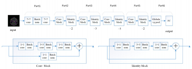
In order to improve the segmentation effect of brain tumor images and address the issue of feature information loss during convolutional neural network (CNN) training, we present an MRI brain tumor segmentation method that leverages an enhanced U-Net architecture. First, the ResNet50 network was used as the backbone network of the improved U-Net, the deeper CNN can improve the feature extraction effect. Next, the Residual Module was enhanced by incorporating the Convolutional Block Attention Module (CBAM). To increase characterization capabilities, focus on important features and suppress unnecessary features. Finally, the cross-entropy loss function and the Dice similarity coefficient are mixed to compose the loss function of the network. To solve the class unbalance problem of the data and enhance the tumor area segmentation outcome. The method's segmentation performance was evaluated using the test set. In this test set, the enhanced U-Net achieved an average Intersection over Union (IoU) of 86.64% and a Dice evaluation score of 87.47%. These values were 3.13% and 2.06% higher, respectively, compared to the original U-Net and R-Unet models. Consequently, the proposed enhanced U-Net in this study significantly improves the brain tumor segmentation efficacy, offering valuable technical support for MRI diagnosis and treatment.

| [1] |
L. Weizman, Y. C. Eldar, D. B. Bashat, Reference‐based MRI, Med. Phys., 43 (2016), 5357–5369. https://doi.org/10.1118/1.4962032 doi: 10.1118/1.4962032

|
| [2] | S. Angelina, L. P. Suresh, S. H. K. Veni, Image segmentation based on genetic algorithm for region growth and region merging, in 2012 International Conference on Computing, Electronics and Electrical Technologies (ICCEET), IEEE, (2012), 970–974. https://doi.org/10.1109/ICCEET.2012.6203833 |
| [3] | Y. Y. Boykov, M. Jolly, Interactive graph cuts for optimal boundary & region segmentation of objects in ND images, in Proceedings Eighth IEEE International Conference on Computer Vision (ICCV), IEEE, (2001), 105–112. https://doi.org/10.1109/ICCV.2001.937505 |
| [4] |
G. C. Lin, W. J. Wang, C. C. Kang, C. M. Wang, Multispectral MR images segmentation based on fuzzy knowledge and modified seeded region growing, Magn. Reson. Imaging, 30 (2012), 230–246. https://doi.org/10.1016/j.mri.2011.09.008 doi: 10.1016/j.mri.2011.09.008
|
| [5] | B. Radhakrishnan, L. P. Suresh, Tumor region extraction using edge detection method in brain MRI images, in 2017 International Conference on Circuit, Power and Computing Technologies (ICCPCT), IEEE, (2017), 1–5. https://doi.org/10.1109/ICCPCT.2017.8074326 |
| [6] |
N. Nabizadeh, M. Kubat, Brain tumors detection and segmentation in MR images: Gabor wavelet vs. statistical features, Comput. Electr. Eng., 45 (2015), 286–301. https://doi.org/10.1016/j.compeleceng.2015.02.007 doi: 10.1016/j.compeleceng.2015.02.007
|
| [7] | W. Deng, X. Wei, D. He, J. Liu, MRI brain tumor segmentation with region growing method based on the gradients and variances along and inside of the boundary curve, in 2010 3rd International Conference on Biomedical Engineering and Informatics, IEEE, (2010), 393–396. https://doi.org/10.1109/BMEI.2010.5639536 |
| [8] |
C. Corte, V. Vapnik, Support vector networks, Mach. Learn., 20 (1995), 273–297. https://doi.org/10.1023/A:1022627411411 doi: 10.1023/A:1022627411411
|
| [9] |
L. Breiman, Random forests, Mach. Learn., 45 (2001), 5–32. https://doi.org/10.1023/A:1010933404324 doi: 10.1023/A:1010933404324
|
| [10] | S. Krinidis, V. Chatzis, A robust fuzzy local information C-means clustering algorithm, in IEEE Transactions on Image Processing, IEEE, (2010), 1328–1337. https://doi.org/10.1109/TIP.2010.2040763 |
| [11] |
A. Ortiz, J. M. Gorriz, J. Ramirez, D. Salas-Gonzalez, Improving MR brain image segmentation using self-organising maps and entropy-gradient clustering, Inf. Sci., 55 (2014), 508–508. https://doi.org/10.1145/383952.384019 doi: 10.1145/383952.384019
|
| [12] |
K. Usman, K. Rajpoot, Brain tumor classification from multi-modality MRI using wavelets and machine learning, Pattern Anal. Appl., 20 (2017), 871–881. https://doi.org/10.1007/s10044-017-0597-8 doi: 10.1007/s10044-017-0597-8
|
| [13] |
Y. Lecun, Y. Bengio, G. Hinton, Deep learning, Nature, 521 (2015), 436–444. https://doi.org/10.1142/S1793351X16500045 doi: 10.1142/S1793351X16500045
|
| [14] | O. R. Neberrger, P. Fischer, T. Brox, U-Net: convolutional networks for biomedical image segmentation, in Medical Image Computing and Computer-Assisted Intervention–MICCAI 2015: 18th International Conference, Munich, Germany, October 5-9, 2015, Proceedings, Part III 18, (2015), 234–241. https://doi.org/10.1007/978-3-319-24574-4_28 |
| [15] | B. S. Vittlkop, S. R. Dhotre, Automatic segmentation of MRI images for brain tumor using unet, in 2019 1st International Conference on Advances in Information Technology (ICAIT), IEEE, (2019), 507–511. https://doi.org/10.1109/ICAIT47043.2019.8987265 |
| [16] | Z. K. Luo, T. Wang, F. F. Ye, U-Net segmentation model of brain tumor MR image based on attention mechanism and multi-view fusion, J. Image Graphics, 26 (2021), 2208–2218. |
| [17] |
R. Sundarasekar, A. Appathurai, Automatic brain tumor detection and classification based on IoT and machine learning techniques, Fluctuation Noise Lett., 21 (2022), 2250030. https://doi.org/10.1142/S0219477522500304 doi: 10.1142/S0219477522500304
|
| [18] |
H. Chen, Z. Qin, Y. Ding, L. Tian, Z. Qin, Brain tumor segmentation with deep convolutional symmetric neural network, Neurocomputing, 392 (2020), 305–313. https://doi.org/10.1016/j.neucom.2019.01.111 doi: 10.1016/j.neucom.2019.01.111
|
| [19] |
Z. Q. Zhu, X. Y. He, G. Q. Qi, Y. Y. Li, B. S. Cong, Y. Liu, Brain tumor segmentation based on the fusion of deep semantics and edge information in multimodal MRI, Inf. Fusion, 91 (2023), 376–387. https://doi.org/10.1016/J.INFFUS.2022.10.022 doi: 10.1016/J.INFFUS.2022.10.022
|
| [20] |
X. Y. He, G. Q. Qi, Z. Q. Zhu, Y. Y. Li, B. S. Cong, L. T. Bai, Medical image segmentation method based on multi-feature interaction and fusion over cloud computing, Simul. Modell. Pract. Theory, 126 (2023), 102769. https://doi.org/10.1016/J.SIMPAT.2023.102769 doi: 10.1016/J.SIMPAT.2023.102769
|
| [21] | Y. Y. Li, Z. Y. Wang, L. Yin, Z. Q. Zhu, G. Q. Qi, Y. Liu, X-Net: a dual encoding–decoding method in medical image segmentation, Visual Comput., 39 (2021), 2223–2233. https://doi.org/10.1007/s00371-021-02328-7 |
| [22] |
Y. Xu, X. Y. He, G. F. Xu, G. Q. Qi, K. Yu, L. Yin, et al., A medical image segmentation method based on multi-dimensional statistical features, Front. Neurosci., 16 (2022), 1009581. https://doi.org/10.3389/FNINS.2022.1009581 doi: 10.3389/FNINS.2022.1009581
|
| [23] | K. W. He, X. Zhang, S. Ren, J. Sun, Deep residual learning for image recognition, in 2016 IEEE Conference on Computer Vision and Pattern Recognition (CVPR), IEEE, (2016), 770–778. https://doi.org/10.1109/CVPR.2016.90 |
| [24] | S. Woo, J. Park, Y. Lee, I. S. Kwon, CBAM: convolutional block attention module, in Proceedings of the European Conference on Computer Vision (ECCV), (2018), 3–19. |
| [25] |
H. B. Yuan, J. J. Zhu, Q. F. Wang, M. Cheng, Z. J. Cai, An improved DeepLab v3+ deep learning network applied to the segmentation of grape leaf black rot spots, Front. Plant Sci., 15 (2022), 281–281. https://doi.org/10.3389/fpls.2022.795410 doi: 10.3389/fpls.2022.795410
|
| [26] |
K. Tomczak, P. Czerwinska, M. Wiznerowicz, The cancer genome atlas: an immeasurable source of knowledge, Contemp. Onkol., 19 (2015), 68–77. https://doi.org/10.5114/wo.2014.47136 doi: 10.5114/wo.2014.47136
|


Figures(8) / Tables(1)

Jiajun Zhu, Rui Zhang, Haifei Zhang. An MRI brain tumor segmentation method based on improved U-Net[J]. Mathematical Biosciences and Engineering, 2024, 21(1): 778-791. doi: 10.3934/mbe.2024033


 DownLoad: