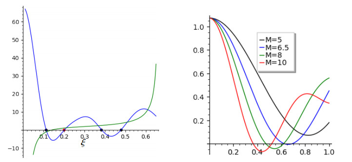
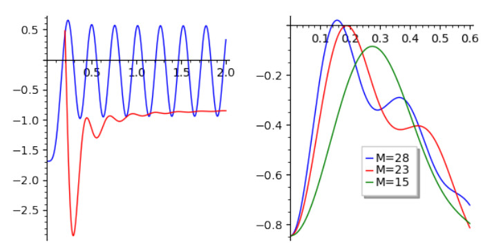
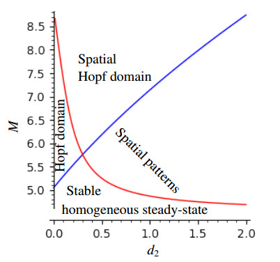
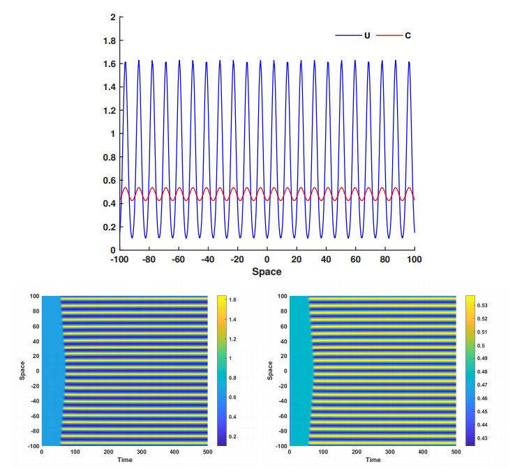
This article investigate a nonlocal reaction-diffusion system of equations modeling virus distribution with respect to their genotypes in the interaction with the immune response. This study demonstrates the existence of pulse solutions corresponding to virus quasi-species. The proof is based on the Leray-Schauder method, which relies on the topological degree for elliptic operators in unbounded domains and a priori estimates of solutions. Furthermore, linear stability analysis of a spatially homogeneous stationary solution identifies the critical conditions for the emergence of spatial and spatiotemporal structures. Finally, numerical simulations are used to illustrate nonlinear dynamics and pattern formation in the nonlocal model.
Citation: Ali Moussaoui, Vitaly Volpert. The influence of immune cells on the existence of virus quasi-species[J]. Mathematical Biosciences and Engineering, 2023, 20(9): 15942-15961. doi: 10.3934/mbe.2023710
This article investigate a nonlocal reaction-diffusion system of equations modeling virus distribution with respect to their genotypes in the interaction with the immune response. This study demonstrates the existence of pulse solutions corresponding to virus quasi-species. The proof is based on the Leray-Schauder method, which relies on the topological degree for elliptic operators in unbounded domains and a priori estimates of solutions. Furthermore, linear stability analysis of a spatially homogeneous stationary solution identifies the critical conditions for the emergence of spatial and spatiotemporal structures. Finally, numerical simulations are used to illustrate nonlinear dynamics and pattern formation in the nonlocal model.

| [1] |
M. Vignuzzi, J. K. Stone, J. J. Arnold, C. E. Cameron, R. Andino, Quasispecies diversity determines pathogenesis through cooperative interactions in a viral population, Nature, 439 (2006), 344–348. https://doi.org/10.1038/nature04388 doi: 10.1038/nature04388

|
| [2] |
M. Vignuzzi, E. Wendt, R. Andino, Engineering attenuated virus vaccines by controlling replication fidelity, Nat. Med., 14 (2008), 154–161. https://doi.org/10.1038/nm1726 doi: 10.1038/nm1726
|
| [3] |
J. Coffin, R. Swanstrom, HIV pathogenesis: dynamics and genetics of viral populations and infected cells, Cold Spring Harb Perspect Med., 3 (2013). https://doi.org/10.1101/cshperspect.a012526 doi: 10.1101/cshperspect.a012526
|
| [4] |
Y. F. Lu, D. B. Goldstein, M. Angrist, G. Cavalleri, Personalized medicine and human genetic diversity, Cold Spring Harb. Perspect. Med., 4 (2014). https://doi.org/10.1101/cshperspect.a008581 doi: 10.1101/cshperspect.a008581
|
| [5] |
N. Echeverria, G. Moratorio, J. Cristina, P. Moreno, Hepatitis C virus genetic variability and evolution, World J. Hepatol., 7 (2015), 831–845. https://doi.org/10.4254/wjh.v7.i6.831 doi: 10.4254/wjh.v7.i6.831
|
| [6] |
T. A. Timofeeva, M. N. Asatryan, A. D. Altstein, B. S. Narodisky, A. L. Gintsburg, N. V. Kaverin, Predicting the Evolutionary Variability of the Influenza A Virus, Acta Naturae, 9 (2017), 48–54. https://doi.org/10.32607/20758251-2017-9-3-48-54 doi: 10.32607/20758251-2017-9-3-48-54
|
| [7] |
N. Bessonov, G. Bocharov, A. Meyerhans, V. Popov, V. Volpert, Existence and dynamics of strains in a nonlocal reaction-diffusion model of viral evolution, SIAM J. Appl. Math., 81 (2021), 107–128. https://doi.org/10.1137/19M1282234 doi: 10.1137/19M1282234
|
| [8] |
Y. Haraguchi, A. Sasaki, Evolutionary pattern of intra-host pathogen antigenic drift: effect of cross-reactivity in immune response, Philos. Trans. R. Soc. Lond. B Biol. Sci., 352 (1997), 11–20. https://doi.org/10.1098/rstb.1997.0002 doi: 10.1098/rstb.1997.0002
|
| [9] |
K. J. Schlesinger, S. P. Stromberg, J. M. Carlson, Coevolutionary immune system dynamics driving pathogen speciation, PLoS One, 9 (2014). https://doi.org/10.1371/journal.pone.0102821 doi: 10.1371/journal.pone.0102821
|
| [10] |
I. M. Rouzine, G. Rozhnova, Antigenic evolution of viruses in host populations, PLoS Pathog., 14 (2018). https://doi.org/10.1371/journal.ppat.1007291 doi: 10.1371/journal.ppat.1007291
|
| [11] |
P. A. Lind, E. Libby, J. Herzog, P. B. Rainey, Predicting mutational routes to new adaptive phenotypes, Elife, 8 (2019). https://doi.org/10.7554/eLife.38822 doi: 10.7554/eLife.38822
|
| [12] |
J. A. de Visser, J. Krug, Empirical fitness landscapes and the predictability of evolution, Nat. Rev. Genet., 15 (2014), 480–490. https://doi.org/10.1038/nrg3744 doi: 10.1038/nrg3744
|
| [13] |
A. Rotem, A. W. R. Serohijos, C. B. Chang, J. T. Wolfe, A. E. Fischer, T. S. Mehoke, et al., Evolution on the biophysical fitness landscape of an RNA virus, Mol. Biol. Evol., 35 (2018), 2390–2400. https://doi.org/10.1093/molbev/msy131 doi: 10.1093/molbev/msy131
|
| [14] |
S. D. Frost, T. Wrin, D. M. Smith, S. L. Kosakovsky Pond, Y. Liu, E. Paxinos, et al., Neutralizing antibody responses drive the evolution of human immunodeficiency virus type 1 envelope during recent HIV infection, Proc. Natl. Acad. Sci., 102 (2005), 18514–18519. https://doi.org/10.1073/pnas.0504658102 doi: 10.1073/pnas.0504658102
|
| [15] |
F. Zanini, V. Puller, J. Brodin, J. Albert, R. A. Neher, In vivo mutation rates and the landscape of fitness costs of HIV-1, Virus Evol., 3 (2017), vex003. https://doi.org/10.1073/pnas.0504658102 doi: 10.1073/pnas.0504658102
|
| [16] |
C. K. Biebricher, M. Eigen, What is a quasispecies?, Curr Top. Microbiol. Immunol., 299 (2006), 1–31. https://doi.org/10.1007/3-540-26397-7-1 doi: 10.1007/3-540-26397-7-1
|
| [17] |
E. Domingo, J. Sheldon, C. Perales, Viral Quasispecies, Evolution Microbiol. Mol. Biol. Rev., 76 (2012), 159–216. https://doi.org/10.1371/journal.pgen.1008271 doi: 10.1371/journal.pgen.1008271
|
| [18] | M. Nowak, R. M. May, Virus Dynamics, in Mathematical Principles of Immunology and Virology, Oxford University Press, 2000. https://doi.org/10.1038/87836 |
| [19] |
M. Kimura, Diffusion models in population genetics, J. Appl. Probability, 1 (1964), 177–232. https://doi.org/10.2307/3211856 doi: 10.2307/3211856
|
| [20] |
A. Sasaki, Evolution of antigen drift/switching: continuously evading pathogens, J. Theor. Biol., 168 (1994), 291–308. https://doi.org/10.1006/jtbi.1994.1110 doi: 10.1006/jtbi.1994.1110
|
| [21] |
N. Bessonov, G. A. Bocharov, C. Leon, V. Popov, V. Volpert, Genotype-dependent virus distribution and competition of virus strains, Math. Mech. Complex Syst., 8 (2020). https://doi.org/10.2140/memocs.2020.8.101 doi: 10.2140/memocs.2020.8.101
|
| [22] |
G. Bocharov, A. Meyerhans, N. Bessonov, S. Trofimchuk, V. Volpert, Interplay between reaction and diffusion processes in governing the dynamics of virus infections, J. Theor. Biol., 457 (2018), 221–236. https://doi.org/10.1016/j.jtbi.2018.08.036 doi: 10.1016/j.jtbi.2018.08.036
|
| [23] |
G. Bocharov, A. Meyerhans, N. Bessonov, S. Trofimchuk, V. Volpert, Modelling the dynamics of virus infection and immune response in space and time, Int. J. Parallel Emergent Distrib. Syst., 34 (2019), 341–355. https://doi.org/10.1080/17445760.2017.1363203 doi: 10.1080/17445760.2017.1363203
|
| [24] | V. Volpert, Elliptic partial differential equations. Volume 2. Reaction-diffusion equations, Birkhäuser, Basel, 2014. http://dml.mathdoc.fr/item/ISBN: ISBN: 978-3-0348-0812-5/ |
| [25] |
C. Leon, I. Kutsenko, V. Volpert, Existence of solutions for a nonlocal reaction-diffusion equation in biomedical applications, Israel J. Math., 248 (2022), 67–93. https://doi.org/10.1007/s11856-022-2294-6 doi: 10.1007/s11856-022-2294-6
|
| [26] | A. Volpert, V. Volpert, Spectrum of elliptic operators and stability of travelling waves, Asymptotic Anal., 23 (2000), 111–134. https://content.iospress.com/articles/asymptotic-analysis/asy392 |
| [27] | J. D. Murray, Mathematical Biology II, Springer-Verlag, Heidelberg, 2002. https://doi.org/10.1007/b98869 |
| [28] |
N. Bessonov, G. Bocharov, A. Meyerhans, V. Popov, V. Volpert, Existence and dynamics of strains in a nonlocal reaction-diffusion model of viral evolution, SIAM J. Appl. Math., 81 (2021), 107–128. https://doi.org/10.1137/19M12822 doi: 10.1137/19M12822
|
| [29] |
L. Segal, V. Volpert, A. Bayliss, Pattern formation in a model of competing populations with nonlocal interactions, Phys. D, 253 (2013), 12–23. https://doi.org/10.1016/j.physd.2013.02.006 doi: 10.1016/j.physd.2013.02.006
|
| [30] |
N. Bessonov, N. Reinberg, M. Banerjee, V. Volpert, The origin of species by means of mathematical modelling, Acta Biotheoretica, 66 (2018), 333–344. https://doi.org/10.1007/s10441-018-9328-9 doi: 10.1007/s10441-018-9328-9
|
| [31] |
N. Bessonov, D. Neverova, V. Popov, V. Volpert, Emergence and competition of virus variants in respiratory viral infections, Front. Immunol., 13 (2023), 945228. https://doi.org/10.3389/fimmu.2022.945228 doi: 10.3389/fimmu.2022.945228
|
Figures(6)

Ali Moussaoui, Vitaly Volpert. The influence of immune cells on the existence of virus quasi-species[J]. Mathematical Biosciences and Engineering, 2023, 20(9): 15942-15961. doi: 10.3934/mbe.2023710


 DownLoad: