Nonlocal multiscale modelling of tumour-oncolytic viruses interactions within a heterogeneous fibrous/non-fibrous extracellular matrix

Abdulhamed Alsisi; Raluca Eftimie; Dumitru Trucu; Abdulhamed Alsisi; Raluca Eftimie; Dumitru Trucu

doi:10.3934/mbe.2022288

Mathematical Biosciences and Engineering

2022, Volume 19, Issue 6: 6157-6185. doi: 10.3934/mbe.2022288

Previous Article Next Article

Research article Special Issues

Nonlocal multiscale modelling of tumour-oncolytic viruses interactions within a heterogeneous fibrous/non-fibrous extracellular matrix

1.
Division of Mathematics, University of Dundee, Dundee DD1 4HN, United Kingdom
2.
Laboratoire Mathematiques de Besançon, UMR-CNRS 6623, Université de Bourgogne Franche-Comté, 16 Route de Gray, Besançon, France

Academic Editor: Sophia Jang

Received: 17 December 2021 Revised: 20 February 2022 Accepted: 07 March 2022 Published: 14 April 2022

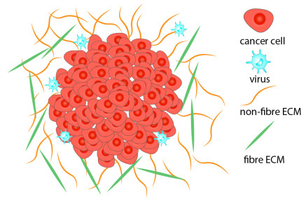
In this study we investigate computationally tumour-oncolytic virus (OV) interactions that take place within a heterogeneous extracellular matrix (ECM). The ECM is viewed as a mixture of two constitutive phases, namely a fibre phase and a non-fibre phase. The multiscale mathematical model presented here focuses on the nonlocal cell-cell and cell-ECM interactions, and how these interactions might be impacted by the infection of cancer cells with the OV. At macroscale we track the kinetics of cancer cells, virus particles and the ECM. At microscale we track (i) the degradation of ECM by matrix degrading enzymes (MDEs) produced by cancer cells, which further influences the movement of tumour boundary; (ii) the re-arrangement of the microfibres that influences the re-arrangement of macrofibres (i.e., fibres at macroscale). With the help of this new multiscale model, we investigate two questions: (i) whether the infected cancer cell fluxes are the result of local or non-local advection in response to ECM density; and (ii) what is the effect of ECM fibres on the the spatial spread of oncolytic viruses and the outcome of oncolytic virotherapy.
- multiscale cancer modelling,
- non-local cell adhesion,
- tumour-oncolytic viruses interactions,
- cancer invasion,
- computational modelling,
- cross cell-cell adhesion,
- extracellular matrix fibres
Citation: Abdulhamed Alsisi, Raluca Eftimie, Dumitru Trucu. Nonlocal multiscale modelling of tumour-oncolytic viruses interactions within a heterogeneous fibrous/non-fibrous extracellular matrix[J]. Mathematical Biosciences and Engineering, 2022, 19(6): 6157-6185. doi: 10.3934/mbe.2022288

Related Papers:

Abstract

In this study we investigate computationally tumour-oncolytic virus (OV) interactions that take place within a heterogeneous extracellular matrix (ECM). The ECM is viewed as a mixture of two constitutive phases, namely a fibre phase and a non-fibre phase. The multiscale mathematical model presented here focuses on the nonlocal cell-cell and cell-ECM interactions, and how these interactions might be impacted by the infection of cancer cells with the OV. At macroscale we track the kinetics of cancer cells, virus particles and the ECM. At microscale we track (i) the degradation of ECM by matrix degrading enzymes (MDEs) produced by cancer cells, which further influences the movement of tumour boundary; (ii) the re-arrangement of the microfibres that influences the re-arrangement of macrofibres (i.e., fibres at macroscale). With the help of this new multiscale model, we investigate two questions: (i) whether the infected cancer cell fluxes are the result of local or non-local advection in response to ECM density; and (ii) what is the effect of ECM fibres on the the spatial spread of oncolytic viruses and the outcome of oncolytic virotherapy.

References

[1]	T. Rozario, D. W. DeSimone, The extracellular matrix in development and morphogenesis: a dynamic view, Dev. Biol., 341 (2010), 126–140. https://doi.org/10.1016/j.ydbio.2009.10.026 doi: 10.1016/j.ydbio.2009.10.026
[2]	B. Yue, Biology of the extracellular matrix: an overview, J. Galucoma, 23 (2015), S20–S23. https://doi.org/10.1097/IJG.0000000000000108 doi: 10.1097/IJG.0000000000000108
[3]	V. Gkretsi, T. Stylianopoulos, Cell adhesion and matrix stiffness: coordinating cancer cell invasion and metastasis, Front. Oncol., 8 (2018), 145. https://doi.org/10.3389/fonc.2018.00145 doi: 10.3389/fonc.2018.00145
[4]	C. Fountzilas, S. Patel, D. Mahalingam, Review: oncolytic virotherapy, updates and future directions, Oncotarget, 8 (2017), 102617–102639.
[5]	H. L. Kaufman, F. J. Kohlhapp, A. Zloza, Oncolytic viruses: a new class of immunotherapy drugs, Nat. Rev. Drug Discov., 14 (2015), 642–662. https://doi.org/10.1038/nrd4663 doi: 10.1038/nrd4663
[6]	J. Pol, G. Kroemer, L. Galluzzi, First oncolytic virus approved for melanoma immunotherapy, Oncoimmunology, 5 (2016), e1115641. https://doi.org/10.1080/2162402X.2015.1115641 doi: 10.1080/2162402X.2015.1115641
[7]	S. J. Russell, K. W. Peng, J. C. Bell, Oncolytic virotherapy, Nat. Biotechnol., 30 (2012), 658–670. https://doi.org/10.1038/nbt.2287 doi: 10.1038/nbt.2287
[8]	J. Wojton, B. Kaur, Impact of tumor microenvironment on oncolytic viral therapy, Cytokine Growth Factor Rev., 21 (2010), 127–134. https://doi.org/10.1016/j.cytogfr.2010.02.014 doi: 10.1016/j.cytogfr.2010.02.014
[9]	N. J. Armstrong, K. J. Painter, J. A. Sherratt, A continuum approach to modelling cell-cell adhesion, J. Theor. Biol., 243 (2006), 98–113. https://doi.org/10.1016/j.jtbi.2006.05.030 doi: 10.1016/j.jtbi.2006.05.030
[10]	A. Gerisch, M. A. Chaplain, Mathematical modelling of cancer cell invasion of tissue: local and non-local models and the effect of adhesion, J. Theor. Biol., 250 (2008), 684–704. https://doi.org/10.1016/j.jtbi.2007.10.026 doi: 10.1016/j.jtbi.2007.10.026
[11]	P. Domschke, D. Trucu, A. Gerisch, M. A. J. Chaplain, Mathematical modelling of cancer invasion: implications of cell adhesion variability for tumour infiltrative growth patterns, J. Theor. Biol., 361 (2014), 41–60. https://doi.org/10.1016/j.jtbi.2014.07.010 doi: 10.1016/j.jtbi.2014.07.010
[12]	J. J. Crivelli, J. Földes, P. S. Kim, J. R. Wares, A mathematical model for cell cycle-specific cancer virotherapy, J. Biol. Dyn., 6 (2012), 104–120. https://doi.org/10.1080/17513758.2011.613486 doi: 10.1080/17513758.2011.613486
[13]	R. Eftimie, J. Dushoff, B. W. Bridle, J. L. Bramson, D. J. Earn, Multi-stability and multi-instability phenomena in a mathematical model of tumor-immune-virus interactions, Bull. Math. Biol., 73 (2011), 2932–2961. https://doi.org/10.1007/s11538-011-9653-5 doi: 10.1007/s11538-011-9653-5
[14]	R. Eftimie, C. K. MacNamara, J. Dushoff, J. L. Bramson, D. J. Earn, Bifurcations and chaotic dynamics in a tumour-immune-virus system, Math. Model. Nat. Phenom., 11 (2016), 65–85. https://doi.org/10.1051/mmnp/201611505 doi: 10.1051/mmnp/201611505
[15]	J. L. Gevertz, J. R. Wares, Developing a minimally structured mathematical model of cancer treatment with oncolytic viruses and dendritic cell injections, Comput. Math. Methods Med., 2018 (2018), 1–14. https://doi.org/10.1155/2018/8760371 doi: 10.1155/2018/8760371
[16]	J. P. W. Heidbuechel, D. Abate-Daga, C. E. Engeland, H. Enderling, Mathematical modeling of oncolytic virotherapy, in Oncolytic Viruses, Humana, New York, (2020), 307–320. https://doi.org/10.1007/978-1-4939-9794-7_21
[17]	M. A. Nowak, R. M. May, Virus Dynamics: Mathematical Principles of Immunology and Virology, Oxford University Press, Oxford, 2000.
[18]	D. Wodarz, Computational modeling approaches to the dynamics of oncolytic viruses, Wiley Interdiscip. Rev. Syst. Biol. Med., 8 (2016), 242–252. https://doi.org/10.1002/wsbm.1332 doi: 10.1002/wsbm.1332
[19]	D. R. Berg, C. P. Offord, I. Kemler, M. K. Ennis, L. Chang, G. Paulik, et al., In vitro and in silico multidimensional modeling of oncolytic tumor virotherapy dynamics, PLOS Comput. Biol., 15 (2019), e1006773. https://doi.org/10.1371/journal.pcbi.1006773 doi: 10.1371/journal.pcbi.1006773
[20]	K. Jacobsen, S. S. Pilyugin, Analysis of a mathematical model for tumor therapy with a fusogenic oncolytic virus, Math. Biosci., 270 (2015), 169–182. https://doi.org/10.1016/j.mbs.2015.02.009 doi: 10.1016/j.mbs.2015.02.009
[21]	J. Malinzi, P. Sibanda, H. Mambili-Mamboundou, Analysis of virotherapy in solid tumor invasion, Math. Biosci., 263 (2015), 102–110. https://doi.org/10.1016/j.mbs.2015.01.015 doi: 10.1016/j.mbs.2015.01.015
[22]	Y. Tao, M. Winkler, Global classical solutions to a doubly haptotactic cross-diffusion system modeling oncolytic virotherapy, J. Differ. Equation, 268 (2020), 4973–4997. https://doi.org/10.1016/j.jde.2019.10.046 doi: 10.1016/j.jde.2019.10.046
[23]	D. Wodarz, A. Hofacre, J. W. Lau, Z. Sun, H. Fan, N. L. Komarova, Complex spatial dynamics of oncolytic viruses in vitro: mathematical and experimental approaches, PLoS Comput. Biol., 8 (2012), e1002547. https://doi.org/10.1371/journal.pcbi.1002547 doi: 10.1371/journal.pcbi.1002547
[24]	A. Alsisi, R. Eftimie, D. Trucu, Non-local multiscale approaches for tumour-oncolytic viruses interactions, Math. Appl. Sci. Eng., 1 (2020), 249–273. https://doi.org/10.5206/mase/10773 doi: 10.5206/mase/10773
[25]	A. Alsisi, R. Eftimie, D. Trucu, Non-local multiscale approach for the impact of go or grow hypothesis on tumour-viruses interactions, Math. Biosci. Eng., 18 (2021), 5252–5284. https://doi.org/10.3934/mbe.2021267 doi: 10.3934/mbe.2021267
[26]	T. Alzahrani, R. Eftimie, D. Trucu, Multiscale modelling of cancer response to oncolytic viral therapy, Math. Biosci., 310 (2019), 76–95. https://doi.org/10.1016/j.mbs.2018.12.018 doi: 10.1016/j.mbs.2018.12.018
[27]	T. Alzahrani, R. Eftimie, D. Trucu, Multiscale moving boundary modelling of cancer interactions with a fusogenic oncolytic virus: the impact of syncytia dynamics, Math. Biosci., 323 (2020), 108296. https://doi.org/10.1016/j.mbs.2019.108296 doi: 10.1016/j.mbs.2019.108296
[28]	L. R. Paiva, C. Binny, S. C. Ferreira, M. L. Martins, A Multiscale mathematical model for oncolytic virotherapy, Cancer Res., 69 (2009), 1205–1211. https://doi.org/10.1158/0008-5472.CAN-08-2173 doi: 10.1158/0008-5472.CAN-08-2173
[29]	L. R. Paiva, H. S. Silva, S. C. Ferreira, M. L. Martins, Multiscale model for the effects of adaptive immunity suppression on the viral therapy of cancer, Phys. Biol., 10 (2013), 025005. https://doi.org/10.1088/1478-3975/10/2/025005 doi: 10.1088/1478-3975/10/2/025005
[30]	D. Trucu, P. Lin, M. A. J. Chaplain, Y. Wang, A multiscale moving boundary model arising in cancer invasion, Multiscale Model. Simul., 11 (2013), 309–335. https://doi.org/10.1137/110839011 doi: 10.1137/110839011
[31]	R. Shuttleworth, D. Trucu, Multiscale modelling of fibres dynamics and cell adhesion within moving boundary cancer invasion, Bull. Math. Biol., 81 (2019), 2176–2219. https://doi.org/10.1007/s11538-019-00598-w doi: 10.1007/s11538-019-00598-w
[32]	N. Bhagavathula, A. W. Hanosh, K. C. Nerusu, H. Appelman, S. Chakrabarty, J. Varani, Regulation of E-cadherin and $\beta$-catenin by Ca2+ in colon carcinoma is dependent on calcium-sensing receptor expression and function, Int. J. Cancer, 121 (2007), 1455–1462. https://doi.org/10.1002/ijc.22858 doi: 10.1002/ijc.22858
[33]	U. Cavallaro, G. Christofori, Cell adhesion in tumor invasion and metastasis: loss of the glue is not enough, Biochim. Biophys. Acta Rev. Cancer, 1552 (2001), 39–45. https://doi.org/10.1016/S0304-419X(01)00038-5 doi: 10.1016/S0304-419X(01)00038-5
[34]	J. D. Humphries, A. Byron, M. J. Humphries, Integrin ligands at a glance, J. Cell Sci., 119 (2006), 3901–3903. https://doi.org/10.1242/jcs.03098 doi: 10.1242/jcs.03098
[35]	K. S. Ko, P. D. Arora, V. Bhide, A. Chen, C. A. McCulloch, Cell-cell adhesion in human fibroblasts requires calcium signaling, J. Cell Sci., 114 (2001), 1155–1167. https://doi.org/10.1242/jcs.114.6.1155 doi: 10.1242/jcs.114.6.1155
[36]	B. P. L. Wijnhoven, W. N. M. Dinjens, M. Pignatelli, E-cadherin-catenin cell-cell adhesion complex and human cancer, Br. J. Surg., 87 (2000), 992–1005. https://doi.org/10.1046/j.1365-2168.2000.01513.x doi: 10.1046/j.1365-2168.2000.01513.x
[37]	M. Chaplain, G. Lolas, Mathematical modelling of cancer invasion of tissue: dynamic heterogeneity, Networks Heterog. Media, 1 (2006), 399–439. https://doi.org/10.3934/nhm.2006.1.399 doi: 10.3934/nhm.2006.1.399
[38]	Z. Gu, F. Liu, E. A. Tonkova, S. Y. Lee, D. J. Tschumperlin, M. B. Brenner, Soft matrix is a natural stimulator for cellular invasiveness, Mol. Biol. Cell, 25 (2014), 457–469. https://doi.org/10.1091/mbc.e13-05-0260 doi: 10.1091/mbc.e13-05-0260
[39]	A. M. Hofer, S. Curci, M. A. Doble, E. M. Brown, D. I. Soybel, Intercellular communication mediated by the extracellular calcium-sensing receptor, Nat. Cell Biol., 2 (2000), 392–398. https://doi.org/10.1038/35017020 doi: 10.1038/35017020
[40]	D. Hanahan, R. A. Weinberg, Hallmarks of cancer: the next generation, Cell, 144 (2011), 646–674. https://doi.org/10.1016/j.cell.2011.02.013 doi: 10.1016/j.cell.2011.02.013
[41]	R. A. Weinberg, The Biology of Cancer, Garland Science, New York, 2006.
[42]	D. Trucu, P. Domschke, A. Gerisch. M. Chaplain, Multiscale computational modelling and analysis of cancer invasion, in Mathematical Models and Methods for Living Systems (eds. L. Preziosi, M. A. J. Chaplain and A. Pugliese), Springer, Cham, (2016), 275–321. https://doi.org/10.1007/978-3-319-42679-2_5
[43]	F. Sabeh, R. Shimizu-Hirota, S. J. Weiss, Protease-dependent versus -independent cancer cell invasion programs: three-dimensional amoeboid movement revisited, J. Cell Biol., 185 (2009), 11–19. https://doi.org/10.1083/jcb.200807195 doi: 10.1083/jcb.200807195
[44]	K. Wolf, S. Alexander, V. Schacht, L. M. Coussens, U. H. von Andrian, J. van Rheenen, et al., Collagen-based cell migration models in vitro and in vivo, Semin. Cell Dev. Biol., 20 (2009), 931–941. https://doi.org/10.1016/j.semcdb.2009.08.005 doi: 10.1016/j.semcdb.2009.08.005
[45]	K. Wolf, Y. I. Wu, Y. Liu, J. Geiger, E. Tam, C. Overall, et al., Multi-step pericellular proteolysis controls the transition from individual to collective cancer cell invasion, Nat. Cell Biol., 9 (2007), 893–904. https://doi.org/10.1038/ncb1616 doi: 10.1038/ncb1616
[46]	B. I. Camara, H. Mokrani, E. Afenya, Mathematical modeling of glioma therapy using oncolytic viruses, Math. Biosci. Eng., 10 (2013), 565–578. https://doi.org/10.3934/mbe.2013.10.565 doi: 10.3934/mbe.2013.10.565
[47]	K. J. Painter, N. J. Armstrong, J. A. Sherratt, The impact of adhesion on cellular invasion processes in cancer and development, J. Theor. Biol., 264 (2010), 1057–1067. https://doi.org/10.1016/j.jtbi.2010.03.033 doi: 10.1016/j.jtbi.2010.03.033
[48]	R. Shuttleworth, D. Trucu, Multiscale dynamics of a heterotypic cancer cell population within a fibrous extracellular matrix, J. Theor. Biol., 486 (2020), 110040. https://doi.org/10.1016/j.jtbi.2019.110040 doi: 10.1016/j.jtbi.2019.110040
[49]	L. Peng, D. Trucu, P. Lin, A. Thompson, M. A. Chaplain, A multiscale mathematical model of tumour invasive growth, Bull. Math. Biol., 79 (2017), 389–429. https://doi.org/10.1007/s11538-016-0237-2 doi: 10.1007/s11538-016-0237-2

Reader Comments

Your name:*

Email:*
© 2022 the Author(s), licensee AIMS Press. This is an open access article distributed under the terms of the Creative Commons Attribution License (http://creativecommons.org/licenses/by/4.0)