Bifurcation analysis and exact solutions for a class of generalized time-space fractional nonlinear Schrödinger equations

Baojian Hong; Baojian Hong

doi:10.3934/mbe.2023643

Mathematical Biosciences and Engineering

2023, Volume 20, Issue 8: 14377-14394. doi: 10.3934/mbe.2023643

Previous Article Next Article

Research article Special Issues

Bifurcation analysis and exact solutions for a class of generalized time-space fractional nonlinear Schrödinger equations

Baojian Hong ^,

Faculty of Mathematical Physics, Nanjing Institute of Technology, Nanjing 211167, China

Academic Editor: Jose M. Rodriguez

Received: 15 April 2023 Revised: 22 June 2023 Accepted: 25 June 2023 Published: 30 June 2023

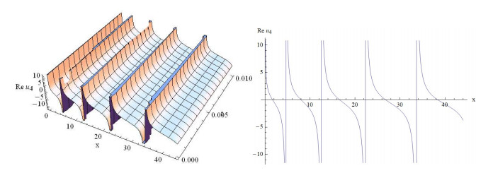
In this work, we focus on a class of generalized time-space fractional nonlinear Schrödinger equations arising in mathematical physics. After utilizing the general mapping deformation method and theory of planar dynamical systems with the aid of symbolic computation, abundant new exact complex doubly periodic solutions, solitary wave solutions and rational function solutions are obtained. Some of them are found for the first time and can be degenerated to trigonometric function solutions. Furthermore, by applying the bifurcation theory method, the periodic wave solutions and traveling wave solutions with the corresponding phase orbits are easily obtained. Moreover, some numerical simulations of these solutions are portrayed, showing the novelty and visibility of the dynamical structure and propagation behavior of this model.
- time-space fractional nonlinear Schrödinger equation,
- general mapping deformation method,
- Caputo fractional derivative,
- bifurcation,
- exact solutions
Citation: Baojian Hong. Bifurcation analysis and exact solutions for a class of generalized time-space fractional nonlinear Schrödinger equations[J]. Mathematical Biosciences and Engineering, 2023, 20(8): 14377-14394. doi: 10.3934/mbe.2023643

Related Papers:

Abstract

In this work, we focus on a class of generalized time-space fractional nonlinear Schrödinger equations arising in mathematical physics. After utilizing the general mapping deformation method and theory of planar dynamical systems with the aid of symbolic computation, abundant new exact complex doubly periodic solutions, solitary wave solutions and rational function solutions are obtained. Some of them are found for the first time and can be degenerated to trigonometric function solutions. Furthermore, by applying the bifurcation theory method, the periodic wave solutions and traveling wave solutions with the corresponding phase orbits are easily obtained. Moreover, some numerical simulations of these solutions are portrayed, showing the novelty and visibility of the dynamical structure and propagation behavior of this model.

References

[1]	I. Podlubny, Fractional Differential Equations, Academic Press, San Diego, 1999.
[2]	R. Hilfer, Applications of Fractional Calculus in Physics, Academic Press, Orlando, 1999.
[3]	M. S. Tavazoei, M. Haeri, S. Jafari, S. Bolouki, M. Siami, Some applications of fractional calculus in suppression of chaotic oscillations, IEEE Trans. Ind. Electron., 55 (2008), 4094–4101. https://doi.org/10.1109/TIE.2008.925774 doi: 10.1109/TIE.2008.925774
[4]	L. Acedo, S. B. Yuste, K. Lindenberg, Reaction front in an a+b→c reaction-subdiffusion process, Phys. Rev. E, 69 (2004), 136–144. https://doi.org/10.1103/PhysRevE.69.036126 doi: 10.1103/PhysRevE.69.036126
[5]	D. A. Benson, S. W. Wheatcraft, M. M. Meerschaert, The fractional-order governing equation of lévy motion, Water Resour. Res., 36 (2000), 1413–1423. https://doi.org/10.1029/2000WR900032 doi: 10.1029/2000WR900032
[6]	J. H. He, Fractal calculus and its geometrical explanation, Results Phys., 10 (2018), 272–276. https://doi.org/10.1016/j.rinp.2018.06.011 doi: 10.1016/j.rinp.2018.06.011
[7]	J. H. He, A modified Li-He's variational principle for plasma, Int. J. Numer. Methods Heat Fluid Flow, 31 (2021), 1369–1372. https://doi.org/10.1108/HFF-06-2019-0523 doi: 10.1108/HFF-06-2019-0523
[8]	D. D. Dai, T. T. Ban, Y. L. Wang, W. Zhang, The piecewise reproducing kernel method for the time variable fractional order advection-reaction-diffusion equations, Therm. Sci., 25 (2021), 1261–1268. https://doi.org/10.2298/TSCI200302021D doi: 10.2298/TSCI200302021D
[9]	Q. T. Ain, J. H. He, N. Anjum, M. Ali, The Fractional complex transform: A novel approach to the time fractional Schrödinger equation, Fractals, 28 (2020), 2050141. https://doi.org/10.1142/S0218348X20501418 doi: 10.1142/S0218348X20501418
[10]	D. C. Lu, B. J. Hong, Bäcklund transformation and n-soliton-like solutions to the combined KdV-Burgers equation with variable coefficients, Int. J. Nonlinear Sci., 1 (2006), 3–10.
[11]	V. A. Matveev, M. A. Salle, Darboux Transformations and Solitons, Heidelberg: Springer Verlag, Berlin, 1991. https://doi.org/10.1007/978-3-662-00922-2
[12]	J. J. Fang, D. S. Mou, H. C. Zhang, Y. Y. Wang, Discrete fractional soliton dynamics of the fractional Ablowitz-Ladik model, Optik, 228 (2021), 166186. https://doi.org/10.1016/j.ijleo.2020.166186 doi: 10.1016/j.ijleo.2020.166186
[13]	B. J. Hong, D. C. Lu, New exact Jacobi elliptic function solutions for the coupled Schrödinger-Boussinesq equations, J. Appl. Math., 2013 (2013), 170835. https://doi.org/10.1155/2013/170835 doi: 10.1155/2013/170835
[14]	D. C. Lu, B. J. Hong, L. X. Tian, New explicit exact solutions for the generalized coupled Hirota-Satsuma KdV system, Comput. Math. Appl., 53 (2007), 1181–1190. https://doi.org/10.1016/j.camwa.2006.08.047 doi: 10.1016/j.camwa.2006.08.047
[15]	B. J. Hong, New Jacobi elliptic functions solutions for the variable-coefficient mKdV equation, Appl. Math. Comput., 215 (2009), 2908–2913. https://doi.org/10.1016/j.amc.2009.09.035 doi: 10.1016/j.amc.2009.09.035
[16]	S. K. Mohanty, O. V. Kravchenko, A. N. Dev, Exact traveling wave solutions of the Schamel Burgers equation by using generalized-improved and generalized G'/G -expansion methods, Results Phys., 33 (2022), 105124. https://doi.org/10.1016/j.rinp.2021.105124 doi: 10.1016/j.rinp.2021.105124
[17]	P. R. Kundu, M. R. A. Fahim, M. E. Islam, M. A. Akbar, The sine-Gordon expansion method for higher-dimensional NLEEs and parametric analysis, Heliyon, 7 (2021), e06459. https://doi.org/10.1016/j.heliyon.2021.e06459 doi: 10.1016/j.heliyon.2021.e06459
[18]	S. M. Mirhosseini-Alizamini, N. Ullah, J. Sabi'u, H. Rezazadeh, M. Inc, New exact solutions for nonlinear Atangana conformable Boussinesq-like equations by new Kudryashov method, Int. J. Modern Phys. B, 35 (2021), 2150163. https://doi.org/10.1142/S0217979221501630 doi: 10.1142/S0217979221501630
[19]	S. Zhang, H. Q. Zhang, Fractional sub-equation method and its applications to nonlinear fractional PDEs, Phys. Lett. A, 375 (2011), 1069–1073. https://doi.org/10.1016/j.physleta.2011.01.029 doi: 10.1016/j.physleta.2011.01.029
[20]	B. Xu, Y. F. Zhang, S. Zhang, Line soliton interactions for shallow ocean-waves and novel solutions with peakon, ring, conical, columnar and lump structures based on fractional KP equation, Adv. Math. Phys., 2021 (2021), 6664039. https://doi.org/10.1155/2021/6664039
[21]	B. Xu, S. Zhang, Riemann-Hilbert approach for constructing analytical solutions and conservation laws of a local time-fractional nonlinear Schrödinger equation, Symmetry, 13 (2021), 13091593. https://doi.org/10.3390/sym13091593 doi: 10.3390/sym13091593
[22]	Y. Y. Gu, L. W. Liao, Closed form solutions of Gerdjikov-Ivanov equation in nonlinear fiber optics involving the beta derivatives, Int. J. Modern Phys. B, 36 (2022), 2250116. https://doi.org/10.1142/S0217979222501168
[23]	Y. Y. Gu, N. Aminakbari, Bernoulli (G'/G)-expansion method for nonlinear Schrödinger equation with third-order dispersion, Modern Phys. Lett. B, 36 (2022), 2250028. https://doi.org/10.1007/s11082-021-02807-0 doi: 10.1007/s11082-021-02807-0
[24]	S. Zhang, Y. Y. Wei, B. Xu, Fractional soliton dynamics and spectral transform of time-fractional nonlinear systems: an concrete example, Complexity, 2019 (2019), 7952871. https://doi.org/10.1155/2019/7952871 doi: 10.1155/2019/7952871
[25]	K. L. Geng, D. S. Mou, C. Q. Dai, Nondegenerate solitons of 2-coupled mixed derivative nonlinear Schrödinger equations, Nonlinear Dyn., 111 (2023), 603–617. https://doi.org/10.1007/s11071-022-07833-5 doi: 10.1007/s11071-022-07833-5
[26]	W. B. Bo, R. R. Wang, Y. Fang, Y. Y. Wang, C. Q. Dai, Prediction and dynamical evolution of multipole soliton families in fractional Schrödinger equation with the PT-symmetric potential and saturable nonlinearity, Nonlinear Dyn., 111 (2023), 1577–1588. https://doi.org/10.1007/s11071-022-07884-8 doi: 10.1007/s11071-022-07884-8
[27]	R. R. Wang, Y. Y. Wang, C. Q. Dai, Influence of higher-order nonlinear effects on optical solitons of the complex Swift-Hohenberg model in the mode-locked fiber laser, Opt. Laser Technol., 152 (2022), 108103. https://doi.org/10.1016/j.optlastec.2022.108103 doi: 10.1016/j.optlastec.2022.108103
[28]	S. L. He, B. A. Malomed, D. Mihalache, X. Peng, X. Yu, Y. J. He, et al., Propagation dynamics of abruptly autofocusing circular Airy Gaussian vortex beams in the fractional Schrödinger equation, Chaos, Solitons Fractals, 142 (2021), 110470. https://doi.org/10.1016/j.chaos.2020.110470 doi: 10.1016/j.chaos.2020.110470
[29]	S. L. He, Z. W. Mo, J. L. Tu, Z. L. Lu, Y. Zhang, X. Peng, et al., Chirped Lommel Gaussian vortex beams in strongly nonlocal nonlinear fractional Schrödinger equations, Results Phys., 42 (2022), 106014. https://doi.org/10.1016/j.rinp.2022.106014 doi: 10.1016/j.rinp.2022.106014
[30]	R. K. Dodd, J. C. Eilbeck, J. D. Gibbon, H. C. Morris, Solitons and Nonlinear Wave Equations, Academic Press, London-New York, 1982.
[31]	M. Levy, Parabolic Equation Methods for Electromagnetic Wave Propagation, Institution of Electrical Engineers (IEE), London, 2000.
[32]	A. Arnold, Numerically absorbing boundary conditions for quantum evolution equations, VLSI Des., 6 (1998), 38298. https://doi.org/10.1155/1998/38298 doi: 10.1155/1998/38298
[33]	Y. S. Kivshar, G. P. Agrawal, Optical Solitons: From Fibers to Photonic Crystals, Academic Press, New York, 2003.
[34]	F. D. Tappert, The Parabolic Approximation Method, Springer, Berlin. https://doi.org/10.1007/3-540-08527-0_5
[35]	M. Hosseininia, M. H. Heydari, C. Cattani, N. Khanna, A wavelet method for nonlinear variable-order time fractional 2D Schrödinger equation, Discrete Contin. Dyn. Syst. Ser. S, 14 (2021), 2273–2295. https://doi.org/10.1016/j.camwa.2019.06.008 doi: 10.1016/j.camwa.2019.06.008
[36]	A. Somayeh, N. Mohammad, Exact solitary wave solutions of the complex nonlinear Schrödinger equations, Opt. Int. J. Light Electron. Opt., 127 (2016), 4682–4688. https://doi.org/10.1016/j.ijleo.2016.02.008 doi: 10.1016/j.ijleo.2016.02.008
[37]	M. A. E. Herzallah, K. A. Gepreel, Approximate solution to the time–space fractional cubic nonlinear Schrödinger equation, Appl. Math. Modell., 36 (2012), 5678–5685. https://doi.org/10.1016/j.apm.2012.01.012 doi: 10.1016/j.apm.2012.01.012
[38]	H. Gündodu, M. F. Gzükzl, Cubic nonlinear fractional Schrödinger equation with conformable derivative and its new travelling wave solutions, J. Appl. Math. Comput. Mech., 20 (2021), 29–41. https://doi.org/10.17512/jamcm.2021.2.03 doi: 10.17512/jamcm.2021.2.03
[39]	A. M. Wazwaz, A study on linear and nonlinear Schrödinger equations by the variational iteration method, Chaos Solitons Fractals, 37 (2008), 1136–1142. https://doi.org/10.1016/j.chaos.2006.10.009 doi: 10.1016/j.chaos.2006.10.009
[40]	A. Hasegawa, F. Tappert, Transmission of stationary nonlinear optical pulses in dispersive dielectric fibers. Ⅱ. Normal dispersion, Appl. Phys. Lett., 23 (1973), 171–172. https://doi.org/10.1063/1.1654836 doi: 10.1063/1.1654836
[41]	A. Ebaid, S. M. Khaled, New types of exact solutions for nonlinear Schrödinger equation with cubic nonlinearity, J. Comput. Appl. Math., 235 (2011), 1984–1992. https://doi.org/10.1016/j.cam.2010.09.024 doi: 10.1016/j.cam.2010.09.024
[42]	A. Demir, M. A. Bayrak, E. Ozbilge, New approaches for the solution of space-time fractional Schrödinger equation, Adv. Differ. Equations, 2020 (2020), 1–21. https://doi.org/10.1186/s13662-020-02581-5 doi: 10.1186/s13662-020-02581-5
[43]	N. A. Kudryashov, Method for finding optical solitons of generalized nonlinear Schrödinger equations, Opt. Int. J. Light Electron. Opt., 261 (2022), 169163. https://doi.org/10.1016/j.ijleo.2022.169163 doi: 10.1016/j.ijleo.2022.169163
[44]	B. Ghanbari, K. S. Nisar, M. Aldhaifallah, Abundant solitary wave solutions to an extended nonlinear Schrödinger equation with conformable derivative using an efficient integration method, Adv. Differ. Equations, 328 (2020), 1–25. https://doi.org/10.1186/s13662-020-02787-7 doi: 10.1186/s13662-020-02787-7
[45]	M. T. Darvishi, M. Najafi, A. M. Wazwaz, Conformable space-time fractional nonlinear (1+1)- dimensional Schrödinger-type models and their traveling wave solutions, Chaos Solitons Fractals, 150 (2021), 111187. https://doi.org/10.1016/j.chaos.2021.111187 doi: 10.1016/j.chaos.2021.111187
[46]	T. Mathanaranjan, Optical singular and dark solitons to the (2+1)-dimensional time-space fractional nonlinear Schrödinger equation, Results Phys., 22 (2021), 103870. https://doi.org/10.1016/j.rinp.2021.103870 doi: 10.1016/j.rinp.2021.103870
[47]	Y. X. Chen, X. Xiao, Z. L. Mei, Optical soliton solutions of the (1+1)-dimensional space-time fractional single and coupled nonlinear Schrödinger equations, Results Phys., 18 (2020), 103211. https://doi.org/10.1016/j.rinp.2020.103211 doi: 10.1016/j.rinp.2020.103211
[48]	E. K. Jaradat, O. Alomari, M. Abudayah, A. Al-Faqih, An approximate analytical solution of the nonlinear Schrödinger equation with harmonic oscillator using homotopy perturbation method and Laplace-Adomian decomposition method, Adv. Math. Phys., 2018 (2018), 1–11. https://doi.org/10.1155/2018/6765021 doi: 10.1155/2018/6765021
[49]	M. G. Sakar, F. Erdogan, A. Yzldzrzm, Variational iteration method for the time-fractional Fornberg-Whitham equation, Comput. Math. Appl., 63 (2012), 1382–1388. https://doi.org/10.1016/j.camwa.2012.01.031 doi: 10.1016/j.camwa.2012.01.031
[50]	G. Jumarie, Table of some basic fractional calculus formulae derived from a modified Riemann-Liouville derivative for non-differentiable functions, Appl. Math. Lett., 22 (2009), 378–385. https://doi.org/10.1016/j.aml.2008.06.003 doi: 10.1016/j.aml.2008.06.003
[51]	B. J. Hong, D. C. Lu, W. Chen, Exact and approximate solutions for the fractional Schrödinger equation with variable coefficients, Adv. Differ. Equations, 2019 (2019), 1–10. https://doi.org/10.1186/s13662-019-2313-z doi: 10.1186/s13662-019-2313-z
[52]	B. J. Hong, D. C. Lu, New exact solutions for the generalized variable-coefficient Gardner equation with forcing term, Appl. Math. Comput., 219 (2012), 2732–2738 https://doi.org/10.1016/j.amc.2012.08.104 doi: 10.1016/j.amc.2012.08.104
[53]	B. J. Hong, New exact Jacobi elliptic functions solutions for the generalized coupled Hirota-Satsuma KdV system, Appl. Math. Comput., 217 (2010), 472–479. https://doi.org/10.1016/j.amc.2010.05.079 doi: 10.1016/j.amc.2010.05.079
[54]	J. H. He, S. K. Elagan, Z. B. Li, Geometrical explanation of the fractional complex transform and derivative chain rule for fractional calculus, Phys. Lett. A, 376 (2012), 257–259. https://doi.org/10.1016/j.physleta.2011.11.030 doi: 10.1016/j.physleta.2011.11.030
[55]	Z. B. Li, J. H. He, Fractional complex transformation for fractional differential equation, Math. Comput. Appl., 15 (2010), 970–973. https://doi.org/10.3390/mca15050970 doi: 10.3390/mca15050970
[56]	A. Ebaid, E. H. Aly, Exact solutions for the transformed reduced Ostrovsky equation via the F-expansion method in terms of Weierstrass-elliptic and Jacobian-elliptic functions, Wave Motion, 49 (2012), 296–308. https://doi.org/10.1016/j.wavemoti.2011.11.003 doi: 10.1016/j.wavemoti.2011.11.003
[57]	M. H. Bashar, S. M. R. Islam, Exact solutions to the (2+1)-Dimensional Heisenberg ferromagnetic spin chain equation by using modifified simple equation and improve F-expansion methods, Phys. Open, 5 (2020), 100027. https://doi.org/10.1016/j.physo.2020.100027 doi: 10.1016/j.physo.2020.100027
[58]	C. Scipio, An invariant set in energy space for supercritical NLS in 1D, J. Math. Anal. Appl., 352 (2009), 634–644. https://doi.org/10.1016/j.jmaa.2008.11.023 doi: 10.1016/j.jmaa.2008.11.023
[59]	L. J. Zhang, P. Y. Yuan, J. L. Fu, C. M. Khalique, Bifurcations and exact traveling wave solutions of the Zakharov-Rubenchik equation, Discrete Contin. Dyn. Syst. S, 13 (2018), 2927–2939. https://doi.org/10.3934/dcdss.2020214 doi: 10.3934/dcdss.2020214
[60]	G. A. Xu, Y. Zhan, J. B. Li, Exact solitary wave and periodic-peakon solutions of the complex Ginzburg-Landau equation: Dynamical system approach, Math. Comput. Simul., 191 (2022), 157–167. https://doi.org/10.1016/j.matcom.2021.08.007 doi: 10.1016/j.matcom.2021.08.007

Reader Comments

Your name:*

Email:*
© 2023 the Author(s), licensee AIMS Press. This is an open access article distributed under the terms of the Creative Commons Attribution License (http://creativecommons.org/licenses/by/4.0)