Optimal real-time power dispatch of power grid with wind energy forecasting under extreme weather

Yixin Zhuo; Ling Li; Jian Tang; Wenchuan Meng; Zhanhong Huang; Kui Huang; Jiaqiu Hu; Yiming Qin; Houjian Zhan; Zhencheng Liang; Yixin Zhuo; Ling Li; Jian Tang; Wenchuan Meng; Zhanhong Huang; Kui Huang; Jiaqiu Hu; Yiming Qin; Houjian Zhan; Zhencheng Liang

doi:10.3934/mbe.2023642

Mathematical Biosciences and Engineering

2023, Volume 20, Issue 8: 14353-14376. doi: 10.3934/mbe.2023642

Previous Article Next Article

Research article

Optimal real-time power dispatch of power grid with wind energy forecasting under extreme weather

1.
Dispatching Control Center of Guangxi Power Grid, Nanning 530000, China
2.
Energy Development Research Institute, China Southern Power Grid, Guangzhou 510000, China
3.
College of Electric Power, South China University of Technology, Guangzhou 510641, China

Academic Editor: Yang Kuang

Received: 20 February 2023 Revised: 04 June 2023 Accepted: 06 June 2023 Published: 30 June 2023

With breakthroughs in the power electronics industry, the stability and rapid power regulation of wind power generation have been improved. Its power generation technology is becoming more and more mature. However, there are still weaknesses in the operation and control of power systems under the influence of extreme weather events, especially in real-time power dispatch. To optimally distribute the power of the regulation resources in a more stable manner, a wind energy forecasting-based power dispatch model with time-control intervals optimization is proposed. In this model, the outage of the wind energy under extreme weather is analyzed by an autoregressive integrated moving average model (ARIMA). Additionally, the other regulation resources are used to balance the corresponding wind power drop and power mismatch. Meanwhile, an algorithm names weighted mean of vectors (INFO) is employed to solve the real-time power dispatch and minimize the power deviation between the power command and real output. Lastly, the performance of the proposed optimal real-time power dispatch is executed in a simulation model with ten regulation resources. The simulation tests show that the combination of ARIMA and INFO can effectively improve the power control performance of the PD-WEF system.
- wind energy forecasting,
- real-time power dispatch,
- extreme weather,
- INFO,
- power outage
Citation: Yixin Zhuo, Ling Li, Jian Tang, Wenchuan Meng, Zhanhong Huang, Kui Huang, Jiaqiu Hu, Yiming Qin, Houjian Zhan, Zhencheng Liang. Optimal real-time power dispatch of power grid with wind energy forecasting under extreme weather[J]. Mathematical Biosciences and Engineering, 2023, 20(8): 14353-14376. doi: 10.3934/mbe.2023642

Related Papers:

Abstract

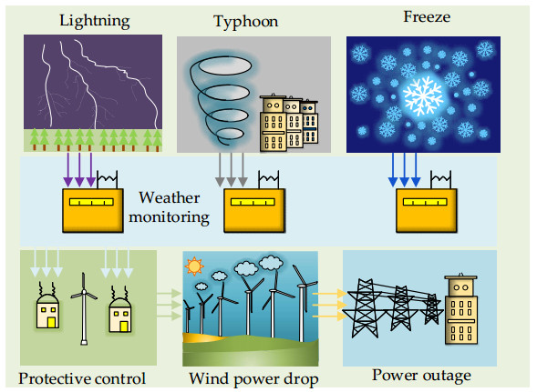
With breakthroughs in the power electronics industry, the stability and rapid power regulation of wind power generation have been improved. Its power generation technology is becoming more and more mature. However, there are still weaknesses in the operation and control of power systems under the influence of extreme weather events, especially in real-time power dispatch. To optimally distribute the power of the regulation resources in a more stable manner, a wind energy forecasting-based power dispatch model with time-control intervals optimization is proposed. In this model, the outage of the wind energy under extreme weather is analyzed by an autoregressive integrated moving average model (ARIMA). Additionally, the other regulation resources are used to balance the corresponding wind power drop and power mismatch. Meanwhile, an algorithm names weighted mean of vectors (INFO) is employed to solve the real-time power dispatch and minimize the power deviation between the power command and real output. Lastly, the performance of the proposed optimal real-time power dispatch is executed in a simulation model with ten regulation resources. The simulation tests show that the combination of ARIMA and INFO can effectively improve the power control performance of the PD-WEF system.

References

[1]	S. A. Yahyai, Y. Charabi, A. Gastli, Review of the use of numerical weather prediction (NWP) models for wind energy assessment, Renewable Sustainable Energy Rev., 14 (2010), 3192–3198. https://doi.org/10.1016/j.rser.2010.07.001 doi: 10.1016/j.rser.2010.07.001
[2]	C. Klessmann, P. Lamers, M. Ragwitz, Design options for cooperation mechanisms under the new European renewable energy directive, Energy Policy, 38 (2010), 4679–4691. https://doi.org/10.1016/j.enpol.2010.04.027 doi: 10.1016/j.enpol.2010.04.027
[3]	R. Lanzafame, M. Messina, Power curve control in micro wind turbine design, Energy, 35 (2010), 556–561. https://doi.org/10.1016/j.energy.2009.10.025 doi: 10.1016/j.energy.2009.10.025
[4]	K. Maslo, Impact of photovoltaics on frequency stability of power system during solar eclipse, IEEE Trans. Power Syst., 31 (2016), 3648–3655. https://doi.org/10.1109/TPWRS.2015.2490245 doi: 10.1109/TPWRS.2015.2490245
[5]	R. Hou, G. Gund, K. Qi, Hybridization design of materials and devices for flexible electrochemical energy storage, Energy Storage Mater., 19 (2019), 212–241. https://doi.org/10.1016/j.ensm.2019.03.002 doi: 10.1016/j.ensm.2019.03.002
[6]	N. Rizoug, T. Mesbahi, R. Sadoun, Development of new improved energy management strategies for electric vehicle battery/supercapacitor hybrid energy storage system, Energy Effic., 11 (2018), 823–843. https://doi.org/10.1007/s12053-017-9602-8 doi: 10.1007/s12053-017-9602-8
[7]	S. Ghosh, S. Kamalasadan, An integrated dynamic modeling and adaptive controller approach for flywheel augmented DFIG based wind system, IEEE Trans. Power Syst., 32 (2017), 2161–2171. https://doi.org/10.1109/TPWRS.2016.2598566 doi: 10.1109/TPWRS.2016.2598566
[8]	J. Deane, E. McKeogh, B. Gallachoir, Derivation of intertemporal targets for large pumped hydro energy storage with stochastic optimization, IEEE Trans. Power Syst., 28 (2013), 2147–2155. https://doi.org/10.1109/TPWRS.2012.2236111 doi: 10.1109/TPWRS.2012.2236111
[9]	M. Koivisto, G. Jonsdottir, P. Sorensen, Combination of meteorological reanalysis data and stochastic simulation for modelling wind generation variability, Renewable Energy, 159 (2020), 991–999. https://doi.org/10.1016/j.renene.2020.06.033 doi: 10.1016/j.renene.2020.06.033
[10]	S. Patra, S. Goswami, Optimum power flow solution using a non-interior point method, Int. J. Elec. Power., 29 (2007), 138–146. https://doi.org/10.1016/j.ijepes.2006.05.008 doi: 10.1016/j.ijepes.2006.05.008
[11]	Y. Liang, J. Juarez, A normalization method for solving the combined economic and emission dispatch problem with meta-heuristic algorithms, Int. J. Electr. Power, 54 (2014), 163–186. https://doi.org/10.1016/j.ijepes.2013.06.022 doi: 10.1016/j.ijepes.2013.06.022
[12]	Y. Zhu, J. Wang, K. Bi, Energy optimal dispatch of the data center microgrid based on stochastic model predictive control, Front. Energy Res., 10 (2022). https://doi.org/10.3389/fenrg.2022.863292 doi: 10.3389/fenrg.2022.863292
[13]	X. Zhang, T. Tan, T. Yu, B. Yang, X. Huang, Bi-objective optimization of real-time AGC dispatch in a performance-based frequency regulation market, CSEE J. Power Energy Syst., 2020 (2020), forthcoming. https://doi.org/10.17775/CSEEJPES.2020.01860
[14]	X. Zhang, C. Li, Z. Li, X. Yin, B. Yang, L. Gan, et al., Optimal mileage-based PV array reconfiguration using swarm reinforcement learning, Energy Convers. Manage., 232 (2021), 113892. https://doi.org/10.1016/j.enconman.2021.113892 doi: 10.1016/j.enconman.2021.113892
[15]	Y. Jiang, M. Liu, J. Li, J. Zhang, Reinforced MCTS for non-intrusive online load identification based on cognitive green computing in smart grid, Math. Biosci. Eng., 19 (2022), 11595–11627. https://doi.org/10.3934/mbe.2022540 doi: 10.3934/mbe.2022540
[16]	S. Wang, C. Zhou, S. Riaz, X. Guo, H. Zaman, A. Mohammad, et al., Adaptive fuzzy-based stability control and series impedance correction for the grid-tied inverter, Math. Biosci. Eng., 20 (2022), 1599–1616. https://doi.org/10.3934/mbe.2023073 doi: 10.3934/mbe.2023073
[17]	Z. Yan, S. Li, W. Gong, An adaptive differential evolution with decomposition for photovoltaic parameter extraction, Math. Biosci. Eng., 18 (2021), 7363–7388. https://doi.org/10.3934/mbe.2021364 doi: 10.3934/mbe.2021364
[18]	J. Li, T. Yu, X. Zhang, F. Li, D. Lin, H. Zhu, Efficient experience replay based deep deterministic policy gradient for AGC dispatch in integrated energy system, Appl. Energy, 285 (2021), 116386. https://doi.org/10.1016/j.apenergy.2020.116386 doi: 10.1016/j.apenergy.2020.116386
[19]	V. Chandran, C. Patil C, A. Manoharan, A. Ghosh, M. G. Sumithra, A. Karthick, et al., Wind power forecasting based on time series model using deep machine learning algorithms, Mater. Today Proc., 47 (2021), 115–126. https://doi.org/10.1016/j.matpr.2021.03.728 doi: 10.1016/j.matpr.2021.03.728
[20]	H. Demolli, A. Dokuz, A. Ecemis, M. Gokcek, Wind power forecasting based on daily wind speed data using machine learning algorithms, Energ. Convers. Manage., 198 (2019), 111823. https://doi.org/10.1016/j.enconman.2019.111823 doi: 10.1016/j.enconman.2019.111823
[21]	J. Sward, T. Ault, K. Zhang, Genetic algorithm selection of the weather research and forecasting model physics to support wind and solar energy integration, Energy, 254 (2022), 124367. https://doi.org/10.1016/j.energy.2022.124367 doi: 10.1016/j.energy.2022.124367
[22]	Y. Qin, K. Li, Z. Liang, B. Lee, F. Zhang, Y. Gu, et al., Hybrid forecasting model based on long short term memory network and deep learning neural network for wind signal, Appl. Energy, 236 (2019), 262–272. https://doi.org/10.1016/j.apenergy.2018.11.063 doi: 10.1016/j.apenergy.2018.11.063
[23]	X. Zhang, Z. Xu, T. Yu, B. Yang, H. Wang, Optimal mileage based AGC dispatch of a Genco, IEEE Trans. Power Syst., 35 (2020), 2516–2526. https://doi.org/10.1109/TPWRS.2020.2966509 doi: 10.1109/TPWRS.2020.2966509
[24]	X. Zhang, C. Li, and B. Xu, Z. Pan, T. Yu, Dropout deep neural network assisted transfer learning for bi-objective Pareto AGC dispatch, IEEE Trans. Power Syst., 38 (2023), 1432–1444. https://doi.org/10.1109/TPWRS.2022.3179372 doi: 10.1109/TPWRS.2022.3179372
[25]	P. Chen, T. Pedersen, B. Bak-Jensen, Z. Chen, ARIMA-based time series model of stochastic wind power generation, IEEE Trans. Power Syst., 25 (2009), 667–676. https://doi.org/10.1109/TPWRS.2009.2033277 doi: 10.1109/TPWRS.2009.2033277
[26]	L. Sobaszek, A. Gola, E. Kozlowski, Predictive scheduling with Markov chains and ARIMA models, Appl. Sci-Basel., 10 (2020), 6121. https://doi.org/10.3390/app10176121 doi: 10.3390/app10176121
[27]	A. Gupta, A. Kumar, Mid-term daily load forecasting using ARIMA, wavelet-ARIMA and machine learning, in 2020 IEEE International Conference on Environment and Electrical Engineering and 2020 IEEE Industrial and Commercial Power Systems Europe (EEEIC/I & CPS Europe), (2020), 1–5. https://doi.org/10.1109/EEEIC/ICPSEurope49358.2020.9160563
[28]	I. Ahmadianfar, A. Heidari, S. Noshadian, H. Chen, A. H. Gandomi, Info: An efficient optimization algorithm based on weighted mean of vectors, Expert Syst. Appl., 195 (2022), 116516. https://doi.org/10.1016/j.eswa.2022.116516 doi: 10.1016/j.eswa.2022.116516
[29]	X. Zhang, T. Yu, B. Yang, L. Jiang, A random forest-assisted fast distributed auction-based algorithm for hierarchical coordinated power control in a large-scale PV power plant, IEEE Trans. Sustain Energy, 12 (2021), 2471–2481. https://doi.org/10.1109/TSTE.2021.3101520 doi: 10.1109/TSTE.2021.3101520
[30]	Z. Laboudi, S. Chikhi, Comparison of genetic algorithm and quantum genetic algorithm, Int. Arab J. Inf. Techn., 9 (2012), 243–249.

Reader Comments

Your name:*

Email:*
© 2023 the Author(s), licensee AIMS Press. This is an open access article distributed under the terms of the Creative Commons Attribution License (http://creativecommons.org/licenses/by/4.0)