The exposure of the Japanese nuclear wastewater incident has shaped online public opinion and has also caused a certain impact on stocks in aquaculture and feed industries. In order to explore the impact of network public opinion caused by public emergencies on relevant stocks, this paper uses the stimulus organism response(SOR) model to construct a framework model of the impact path of network public opinion on the financial stock market, and it uses emotional analysis, LDA and grounded theory methods to conduct empirical analysis. The study draws a new conclusion about the impact of online public opinion on the performance of relevant stocks in the context of the nuclear waste water incident in Japan. The positive change of media sentiment will lead to the decline of stock returns and the increase of volatility. The positive change of public sentiment will lead to the decline of stock returns in the current period and the increase of stock returns in the lag period. At the same time, we have proved that media attention, public opinion theme and prospect theory value have certain influences on stock performance in the context of the Japanese nuclear wastewater incident. The conclusion shows that after the public emergency, the government and investors need to pay attention to the changes of network public opinion caused by the event, so as to avoid the possible stock market risks.
Citation: Wei Hong, Yiting Gu, Linhai Wu, Xujin Pu. Impact of online public opinion regarding the Japanese nuclear wastewater incident on stock market based on the SOR model[J]. Mathematical Biosciences and Engineering, 2023, 20(5): 9305-9326. doi: 10.3934/mbe.2023408
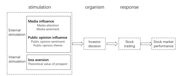
The exposure of the Japanese nuclear wastewater incident has shaped online public opinion and has also caused a certain impact on stocks in aquaculture and feed industries. In order to explore the impact of network public opinion caused by public emergencies on relevant stocks, this paper uses the stimulus organism response(SOR) model to construct a framework model of the impact path of network public opinion on the financial stock market, and it uses emotional analysis, LDA and grounded theory methods to conduct empirical analysis. The study draws a new conclusion about the impact of online public opinion on the performance of relevant stocks in the context of the nuclear waste water incident in Japan. The positive change of media sentiment will lead to the decline of stock returns and the increase of volatility. The positive change of public sentiment will lead to the decline of stock returns in the current period and the increase of stock returns in the lag period. At the same time, we have proved that media attention, public opinion theme and prospect theory value have certain influences on stock performance in the context of the Japanese nuclear wastewater incident. The conclusion shows that after the public emergency, the government and investors need to pay attention to the changes of network public opinion caused by the event, so as to avoid the possible stock market risks.

| [1] |
B. Wang, S. Zhang, J. Dong, Y. Li, Y. Jin, H. Xiao, et al., Ambient temperature structures the gut microbiota of zebrafish to impact the response to radioactive pollution, Environ. Pollut., 293 (2022), 118539. https://doi.org/10.1016/j.envpol.2021.118539 doi: 10.1016/j.envpol.2021.118539

|
| [2] |
K. Liu, J. Zhou, D. Dong, Improving stock price prediction using the long short-term memory model combined with online social networks, J. Behav. Exp. Finance, 30 (2021). https://doi.org/10.1016/j.jbef.2021.100507 doi: 10.1016/j.jbef.2021.100507
|
| [3] |
Y. Lv, J. Piao, B. Li, M. Yang, Does online investor sentiment impact stock returns? Evidence from the Chinese stock market, Appl. Econ. Lett., 29 (2022), 1434–1438. https://doi.org/10.1080/13504851.2021.1937490 doi: 10.1080/13504851.2021.1937490
|
| [4] |
G. Huberman, T. Regev, Contagious speculation and a cure for cancer: A nonevent that made stock prices soar, J. Finance, 56 (2001), 387–396. https://doi.org/10.1111/0022-1082.00330 doi: 10.1111/0022-1082.00330
|
| [5] |
U. Bhattacharya, N. Galpin, R. Ray, X. Yu, The role of the media in the internet IPO bubble, J. Finance Quant. Anal., 44 (2009), 657–682. https://doi.org/10.1017/S0022109009990056 doi: 10.1017/S0022109009990056
|
| [6] |
H. J. V. Heerde, E. Gijsbrechts, K. Pauwels, Fanning the flames? how media coverage of a price war affects retailers, consumers, and investors, J. Mark. Res., 52 (2015), 674–693. https://doi.org/10.1509/jmr.13.0260 doi: 10.1509/jmr.13.0260
|
| [7] |
L. Fang, J. Peress, Media coverage and the cross-section of stock returns, J. Finance, 64 (2009), 2023–2052. https://doi.org/10.1111/j.1540-6261.2009.01493.x doi: 10.1111/j.1540-6261.2009.01493.x
|
| [8] |
P. C. Tetlock, Giving content to investor sentiment: The role of media in the stock market, J. Finance, 62 (2007), 1139–1168. https://doi.org/10.1111/j.1540-6261.2007.01232.x doi: 10.1111/j.1540-6261.2007.01232.x
|
| [9] | J. Engelberg, Costly information processing: evidence from earnings announcements, AFA 2009 San Francisco Meetings Paper, 2008. http://dx.doi.org/10.2139/ssrn.1107998. |
| [10] |
H. Du, J. Hao, F. He, W. Xi, Media sentiment and cross-sectional stock returns in the Chinese stock market, Res. Int. Bus. Finance, 60 (2022), 101590, https://doi.org/10.1016/j.ribaf.2021.101590 doi: 10.1016/j.ribaf.2021.101590
|
| [11] | M. W. Uhl, The Long-run impact of sentiment on stock returns, Working Paper, 2011. |
| [12] |
M. T. Suleman, Stock market reaction to good and bad political news, Asian J. Finance Account., 4 (2012), 299–312. https://doi.org/10.5296/ajfa.v4i1.1705 doi: 10.5296/ajfa.v4i1.1705
|
| [13] |
G. W. Brown, M. T. Cliff., Investor sentiment and the near-term stock market, J. Empir. Finance, 11 (2004), 1–27. https://doi.org/10.1016/j.jempfin.2002.12.001 doi: 10.1016/j.jempfin.2002.12.001
|
| [14] |
J. Wurgler, M. Baker, Investor sentiment and the cross-section of stock returns, J. Finance, 61 (2006), 1645–1680. https://doi.org/10.1111/j.1540-6261.2006.00885.x doi: 10.1111/j.1540-6261.2006.00885.x
|
| [15] |
F. M. Statman, Investor sentiment and stock returns, Finance Anal. J., 56 (2000), 16–23. https://doi.org/10.2469/faj.v56.n2.2340 doi: 10.2469/faj.v56.n2.2340
|
| [16] |
Z. Li, S. Wang, M. Hu, International investor sentiment and stock returns: Evidence from China, Invest. Anal. J., 50 (2021), 60–76. https://doi.org/10.1080/10293523.2021.1876968 doi: 10.1080/10293523.2021.1876968
|
| [17] |
Y. Kim, K. Y. Lee, Impact of investor sentiment on stock returns, Asia-Pac. J. Finance Stud., 51 (2022), 132–162. https://doi.org/10.1111/ajfs.12362 doi: 10.1111/ajfs.12362
|
| [18] |
T. Renault, Intraday online investor sentiment and return patterns in the US stock market, J. Bank Finance, 84 (2017), 25–40. https://doi.org/10.1016/j.jbankfin.2017.07.002 doi: 10.1016/j.jbankfin.2017.07.002
|
| [19] |
E. Bartov, L. Faurel, P. S. Mohanram, Can twitter help predict firm-level earnings and stock returns?, Account. Rev., 93 (2018), 25–57. https://doi.org/10.2308/accr-51865 doi: 10.2308/accr-51865
|
| [20] | Y. Shynkevich, T. M. Mcginnity, S. Coleman, A. Belatreche, Stock price prediction based on stock-specific and sub-industry-specific news articles, in 2015 International Joint Conference on Neural Networks (IJCNN), (2015), 1–8. https://doi.org/10.1109/IJCNN.2015.7280517 |
| [21] | H. Yun, G. Sim, J. Seok, Stock prices prediction using the title of newspaper articles with Korean natural language processing, in 2019 International Conference on Artificial Intelligence in Information and Communication (ICAⅡC), (2019). https://doi.org/10.1109/ICAⅡC.2019.8668996 |
| [22] |
M. Zhang, J. Yang, M. Wan, X. Zhang, J. Zhou., Predicting long-term stock movements with fused textual features of Chinese research reports, Expert Syst. Appl., 210 (2022), 118312. https://doi.org/10.1016/j.eswa.2022.118312 doi: 10.1016/j.eswa.2022.118312
|
| [23] |
N. Barberis, M. Huang, Stock as lotteries: The implications of probability weighting for security prices, Am. Econ. Rev., 98 (2008), 2066–2100. https://doi.org/10.1257/aer.98.5.2066 doi: 10.1257/aer.98.5.2066
|
| [24] |
B. Boyer, T. Mitton, K. Vorkink, Expected idiosyncratic skewness, Rev. Finance Stud., 23 (2010), 169–202. https://doi.org/10.1093/rfs/hhp041 doi: 10.1093/rfs/hhp041
|
| [25] |
T. G. Bali, N. Cakici, R. F. Whitelaw, Maxing out: Stock as lotteries and the cross-section of expected returns, J. Finance Econ., 99 (2011), 427–446. https://doi.org/10.1016/j.jfineco.2010.08.014 doi: 10.1016/j.jfineco.2010.08.014
|
| [26] |
J. Conrad, R. F. Dittmar, E. Ghysels, Ex ante skewness and expected stock returns, J. Finance, 68 (2013), 85–124. https://doi.org/10.1111/j.1540-6261.2012.01795.x doi: 10.1111/j.1540-6261.2012.01795.x
|
| [27] |
N. Barberis, A. Mukherjee, B. Wang, Prospect theory and stock returns: An empirical test, Rev. Finance Stud., 29 (2016), 3068–3107. https://doi.org/10.1093/rfs/hhw049 doi: 10.1093/rfs/hhw049
|
| [28] |
J. Wang, C. Wu, X. Zhong, Prospect theory and stock returns: Evidence from foreign share markets, Pac.-Basin Finance J., 69 (2021), 101644. https://doi.org/10.1016/j.pacfin.2021.101644 doi: 10.1016/j.pacfin.2021.101644
|
| [29] |
A. J. N. Junior, M. C. Klotzle, L. E. T. Brandão, A. C. F. Pinto, Prospect theory and narrow framing bias: Evidence from emerging markets, Q. Rev. Econ. Finance, 80 (2021), 90–101. https://doi.org/10.1016/j.qref.2021.01.016 doi: 10.1016/j.qref.2021.01.016
|
| [30] |
X. Yang, D. Gu, J. Wu, C. Liang, Y. Ma, J. Li, Factors influencing health anxiety: The stimulus–organism-response model perspective, Internet Res., 31 (2021), 2033–2054. https://doi.org/10.1108/INTR-10-2020-0604 doi: 10.1108/INTR-10-2020-0604
|
| [31] |
Z. Tang, M. Warkentin, L. Wu, Understanding employees' energy saving behavior from the perspective of stimulus-organism-responses, Resour. Conserv. Recycl., 140 (2019), 216–223. https://doi.org/10.1016/j.resconrec.2018.09.030 doi: 10.1016/j.resconrec.2018.09.030
|
| [32] |
B. J. Bushee, J. E. Core, W. Guay, S. Hamm, The role of the business press as an information intermediary, J. Account. Res., 48 (2010), 1–19. https://doi.org/10.1111/j.1475-679X.2009.00357.x doi: 10.1111/j.1475-679X.2009.00357.x
|
| [33] |
Z. Da, J. Engelberg, P. J. Gao, In search of attention, J. Finance, 66 (2011), 1461–1499. https://doi.org/10.1111/j.1540-6261.2011.01679.x doi: 10.1111/j.1540-6261.2011.01679.x
|
| [34] |
F. Comiran, T. Fedyk, J. Ha, Accounting quality and media attention around seasoned equity offerings, Int. J. Account. Inf. Manage., 26 (2017), 443–462. https://doi.org/10.1108/IJAIM-02-2017-0029 doi: 10.1108/IJAIM-02-2017-0029
|
| [35] |
W. S. Chan., Stock price reaction to news and no-news: drift and reversal after headlines, J. Finance Econ., 70 (2003), 223–260. https://doi.org/10.1016/S0304-405X(03)00146-6 doi: 10.1016/S0304-405X(03)00146-6
|
| [36] |
P. C. Tetlock, M. Saar-Tsechansky, S. Macskassy, More than words: Quantifying language to measure firms' fundamentals, J. Finance, 63 (2008), 1437–1467. https://doi.org/10.1111/j.1540-6261.2008.01362.x doi: 10.1111/j.1540-6261.2008.01362.x
|
| [37] |
P. Jiao, A. Veiga, A. Walther, Social media, news media and the stock market, J. Econ. Behav. Organ., 176 (2020), 63–90. https://doi.org/10.1016/j.jebo.2020.03.002 doi: 10.1016/j.jebo.2020.03.002
|
| [38] |
T. Huang, X. Zhang, Industry-level media tone and the cross-section of stock returns, Int. Rev. Econ. Finance, 77 (2021), 59–77. https://doi.org/10.1016/j.iref.2021.09.002 doi: 10.1016/j.iref.2021.09.002
|
| [39] |
Y. He, L. Qu, R. Wei, X. Zhao, Media-based investor sentiment and stock returns: A textual analysis based on newspapers, Appl. Econ., 54 (2022), 774–792. https://doi.org/10.1080/00036846.2021.1966369 doi: 10.1080/00036846.2021.1966369
|
| [40] |
W. Wang, C. Su, D. Duxbury, The conditional impact of investor sentiment in global stock markets: A two-channel examination, J. Bank Finance, 138 (2022), 106458. https://doi.org/10.1016/j.jbankfin.2022.106458 doi: 10.1016/j.jbankfin.2022.106458
|
| [41] |
R. B. Cohen, C. Polk, T. Vuolteenaho, The price is (almost) right, J. Finance, 64 (2009), 2739–2782. https://doi.org/10.1111/j.1540-6261.2009.01516.x doi: 10.1111/j.1540-6261.2009.01516.x
|
| [42] |
Z. Da, J. Engelberg, P. Gao, The sum of all FEARS investor sentiment and asset prices, Rev. Finance Stud., 28 (2015), 1–32. https://doi.org/10.1093/rfs/hhu072 doi: 10.1093/rfs/hhu072
|
| [43] |
H. Yang, D. Ryu, D. Ryu, Investor sentiment, asset returns and firm characteristics: Evidence from the Korean stock market, Invest. Anal. J., 46 (2017), 1–16. https://doi.org/10.1080/10293523.2016.1277850 doi: 10.1080/10293523.2016.1277850
|
| [44] |
J. Li, Y. Zhang, L. Wang, Information transmission between large shareholders and stock volatility, N. Am. Econ. Finance, 58 (2021), 101551. https://doi.org/10.1016/j.najef.2021.101551 doi: 10.1016/j.najef.2021.101551
|
| [45] |
M. Ammann, R. Frey, M. Verhofen, Do newspaper articles predict aggregate stock returns?, J. Behav. Finance, 15 (2014), 195–213. https://doi.org/10.1080/15427560.2014.941061 doi: 10.1080/15427560.2014.941061
|
| [46] | F. Wong, Z. Liu, M. Chiang, Stock market prediction from WSJ: text mining via sparse matrix factorization, in Proceedings of the 2014 IEEE International Conference on Data, (2014), 430–439. https://doi.org/10.48550/arXiv.1406.7330 |
| [47] |
N. C. Barberis, Thirty years of prospect theory in economics: A review and assessment, J. Econ. Perspect., 27 (2013), 173–195. https://doi.org/10.1257/jep.27.1.173 doi: 10.1257/jep.27.1.173
|
| [48] | D. Kahneman, A. Tversky, Prospect theory: An analysis of decision under risk, Econometrica, 47 (1979), 263–291. http://www.jstor.org/stable/1914185 |
| [49] |
H. Chen, P. De, Y. Hu, B. H. Hwang, Wisdom of crowds: The value of stock opinions transmitted through social media, Rev. Finance Stud., 27 (2013), 1367–1403. https://doi.org/10.1093/rfs/hhu001 doi: 10.1093/rfs/hhu001
|


Figures(3) / Tables(7)

Wei Hong, Yiting Gu, Linhai Wu, Xujin Pu. Impact of online public opinion regarding the Japanese nuclear wastewater incident on stock market based on the SOR model[J]. Mathematical Biosciences and Engineering, 2023, 20(5): 9305-9326. doi: 10.3934/mbe.2023408


 DownLoad: