Dynamics of a stochastic hepatitis B virus transmission model with media coverage and a case study of China

Jiying Ma; Shasha Ma; Jiying Ma; Shasha Ma

doi:10.3934/mbe.2023145

Mathematical Biosciences and Engineering

2023, Volume 20, Issue 2: 3070-3098. doi: 10.3934/mbe.2023145

Previous Article Next Article

Research article

Dynamics of a stochastic hepatitis B virus transmission model with media coverage and a case study of China

Jiying Ma ^,,
Shasha Ma

College of Science, University of Shanghai for Science and Technology, Shanghai 200093, China
Academic editor: Hao Wang

Received: 19 September 2022 Revised: 03 November 2022 Accepted: 08 November 2022 Published: 01 December 2022

Hepatitis B virus (HBV) infection is a global public health problem and there are $ 257 $ million people living with chronic HBV infection throughout the world. In this paper, we investigate the dynamics of a stochastic HBV transmission model with media coverage and saturated incidence rate. Firstly, we prove the existence and uniqueness of positive solution for the stochastic model. Then the condition on the extinction of HBV infection is obtained, which implies that media coverage helps to control the disease spread and the noise intensities on the acute and chronic HBV infection play a key role in disease eradication. Furthermore, we verify that the system has a unique stationary distribution under certain conditions, and the disease will prevail from the biological perspective. Numerical simulations are conducted to illustrate our theoretical results intuitively. As a case study, we fit our model to the available hepatitis B data of mainland China from 2005 to 2021.
- hepatitis B virus,
- media coverage,
- extinction,
- stationary distribution,
- numerical simulation
Citation: Jiying Ma, Shasha Ma. Dynamics of a stochastic hepatitis B virus transmission model with media coverage and a case study of China[J]. Mathematical Biosciences and Engineering, 2023, 20(2): 3070-3098. doi: 10.3934/mbe.2023145

Related Papers:

Abstract

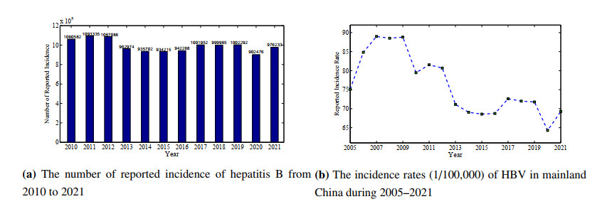
Hepatitis B virus (HBV) infection is a global public health problem and there are $ 257 $ million people living with chronic HBV infection throughout the world. In this paper, we investigate the dynamics of a stochastic HBV transmission model with media coverage and saturated incidence rate. Firstly, we prove the existence and uniqueness of positive solution for the stochastic model. Then the condition on the extinction of HBV infection is obtained, which implies that media coverage helps to control the disease spread and the noise intensities on the acute and chronic HBV infection play a key role in disease eradication. Furthermore, we verify that the system has a unique stationary distribution under certain conditions, and the disease will prevail from the biological perspective. Numerical simulations are conducted to illustrate our theoretical results intuitively. As a case study, we fit our model to the available hepatitis B data of mainland China from 2005 to 2021.

References

[1]	L. Zou, W. Zhang, S. Ruan, Modeling the transmission dynamics and control of hepatitis B virus in China, J. Theor. Biol., 262 (2010), 330–338. https://doi.org/10.1016/j.jtbi.2009.09.035 doi: 10.1016/j.jtbi.2009.09.035
[2]	World health organization, Hepatitis B, Key facts, 2022. Available from: https://www.who.int/news-room/fact-sheets/detail/hepatitis-b
[3]	Chinese Center for Disease Control and Prevention, Chinese Center for Disease Control and Prevention, 2022. Available from: https://www.chinacdc.cn
[4]	R. M. Anderson, R. M. May, Infectious Disease of Humans: Dynamics and Control, Oxford University Press, Oxford, 1991.
[5]	S. Zhao, Z. Xu, Y. Lu, A mathematical model of hepatitis B virus transmission and its application for vaccination strategy in China, Int. J. Epidemiol., 29 (2000), 744–752. https://doi.org/10.1093/ije/29.4.744 doi: 10.1093/ije/29.4.744
[6]	L. Zou, S. Ruan, W. Zhang, On the sexual transmission dynamics of hepatitis B virus in China, J. Theor. Biol., 369 (2015), 1–12. https://doi.org/10.1016/j.jtbi.2015.01.005 doi: 10.1016/j.jtbi.2015.01.005
[7]	T. Zhang, K. Wang, X. Zhang, Modeling and analyzing the transmission dynamics of HBV epidemic in Xinjiang, China, PLoS ONE, 10 (2015), e0138765. https://doi.org/10.1371/journal.pone.0138765 doi: 10.1371/journal.pone.0138765
[8]	A. Din, Y. Li, Mathematical analysis of a new nonlinear stochastic hepatitis B epidemic model with vaccination effect and a case study, Eur. Phys. J. Plus, 137 (2022), 558. https://doi.org/10.1140/epjp/s13360-022-02748-x doi: 10.1140/epjp/s13360-022-02748-x
[9]	T. Khan, A. Khan, G. Zaman, The extinction and persistence of the stochastic hepatitis B epidemic model, Chaos Soliton Fract., 108 (2018), 123–128. https://doi.org/10.1016/j.chaos.2018.01.036 doi: 10.1016/j.chaos.2018.01.036
[10]	T. Khan, I. H. Jung, G. Zaman, A stochastic model for the transmission dynamics of hepatitis B virus, J. Biol. Dyn., 13 (2019), 328–344. https://doi.org/10.1080/17513758.2019.1600750 doi: 10.1080/17513758.2019.1600750
[11]	L. Liu, D. Jiang, T. Hayat, B. Ahmad, Dynamics of a hepatitis B model with saturated incidence, Acta Math. Sci., 38 (2018), 1731–1750. https://doi.org/10.1016/S0252-9602(18)30842-7 doi: 10.1016/S0252-9602(18)30842-7
[12]	Z. Wang, C. T. Bauch, S. Bhattacharyya, A. d'Onofrio, P. Manfredi, M. Perc, et al., Statistical physics of vaccination, Phys. Rep., 664 (2016), 1–113. https://doi.org/10.1016/j.physrep.2016.10.006 doi: 10.1016/j.physrep.2016.10.006
[13]	S. Wang, M. Hao, Z. Pan, J. Lei, X. Zou, Data-driven multi-scale mathematical modeling of SARS-CoV-2 infection reveals heterogeneity among COVID-19 patients, PLoS Comput. Biol., 17 (2021), e1009587. https://doi.org/10.1371/journal.pcbi.1009587 doi: 10.1371/journal.pcbi.1009587
[14]	F. A. Rihan, H. J. Alsakaji, Analysis of a stochastic HBV infection model with delayed immune response, Math. Biosci. Eng., 18 (2021), 5194–5220. https://doi.org/10.3934/mbe.2021264 doi: 10.3934/mbe.2021264
[15]	T. Luzyanina, G. Bocharov, Stochastic modeling of the impact of random forcing on persistent hepatitis B virus infection, Math. Comput. Simul., 96 (2014), 54–65. https://doi.org/10.1016/j.matcom.2011.10.002 doi: 10.1016/j.matcom.2011.10.002
[16]	X. Wang, Y. Tan, Y. Cai, K. Wang, W. Wang, Dynamics of a stochastic HBV infection model with cell-to-cell transmission and immune response, Math. Biosci. Eng., 18 (2021), 616–642. https://doi.org/10.3934/mbe.2021034 doi: 10.3934/mbe.2021034
[17]	F. Mohajerani, B. Tyukodi, C. J. Schlicksup, J. A. Hadden-Perilla, A. Zlotnick, M. F. Hagan, Multiscale modeling of hepatitis B virus capsid assembly and its dimorphism, ACS Nano, 16 (2022), 13845–13859. https://doi.org/10.1021/acsnano.2c02119 doi: 10.1021/acsnano.2c02119
[18]	Y. Cai, Y. Kang, M. Banerjee, W. Wang, A stochastic SIRS epidemic model with infectious force under intervention strategies, J. Differ. Equations, 259 (2015), 7463–7502. https://doi.org/10.1016/j.jde.2015.08.024 doi: 10.1016/j.jde.2015.08.024
[19]	J. Cui, Y. Sun, H. Zhu, The impact of media on the control of infectious diseases, J. Dyn. Differ. Equations, 20 (2008), 31–53. https://doi.org/10.1007/s10884-007-9075-0 doi: 10.1007/s10884-007-9075-0
[20]	J. Cui, X. Tao, H. Zhu, An SIS infection model incorporating media coverage, Rocky Mountain J. Math., 38 (2008), 1323–1334. https://doi.org/10.1216/RMJ-2008-38-5-1323 doi: 10.1216/RMJ-2008-38-5-1323
[21]	Y. Zhao, L. Zhang, S. Yuan, The effect of media coverage on threshold dynamics for a stochastic SIS epidemic model, Phys. A, 512 (2018), 248–260. https://doi.org/10.1016/j.physa.2018.08.113 doi: 10.1016/j.physa.2018.08.113
[22]	W. Guo, Y. Cai, Q. Zhang, W. Wang, Stochastic persistence and stationary distribution in an SIS epidemic model with media coverage, Phys. A, 492 (2018), 2220–2236. https://doi.org/10.1016/j.physa.2017.11.137 doi: 10.1016/j.physa.2017.11.137
[23]	Y. Zhang, K. Fan, S. Gao, Y. Liu, S. Chen, Ergodic stationary distribution of a stochastic SIRS epidemic model incorporating media coverage and saturated incidence rate, Phys. A, 514 (2019), 671–685. https://doi.org/10.1016/j.physa.2018.09.124 doi: 10.1016/j.physa.2018.09.124
[24]	W. Liu, Q. Zheng, A stochastic sis epidemic model incorporating media coverage in a two patch setting, Appl. Math. Comput., 262 (2015), 160–168. https://doi.org/10.1016/j.amc.2015.04.025 doi: 10.1016/j.amc.2015.04.025
[25]	M. A. Khan, S. Islam, G. Zaman, Media coverage campaign in Hepatitis B transmission model, Appl. Math. Comput., 331 (2018), 378–393. https://doi.org/10.1016/j.amc.2018.03.029 doi: 10.1016/j.amc.2018.03.029
[26]	D. Li, J. Cui, M. Liu, S. Liu, The evolutionary dynamics of stochastic epidemic model with nonlinear incidence rate, Bull. Math. Biol., 77 (2015), 1705–1743. https://doi.org/10.1007/s11538-015-0101-9 doi: 10.1007/s11538-015-0101-9
[27]	Q. Liu, D. Jiang, Stationary distribution and extinction of a stochastic SIR model with nonlinear perturbation, Appl. Math. Lett., 73 (2017), 8–15. https://doi.org/10.1016/j.aml.2017.04.021 doi: 10.1016/j.aml.2017.04.021
[28]	W. Wang, Y. Cai, J. Li, Z. Gui, Periodic behavior in a FIV model with seasonality as well as environment fluctuations, J. Franklin Inst., 354 (2017), 7410–7428. https://doi.org/10.1016/j.jfranklin.2017.08.034 doi: 10.1016/j.jfranklin.2017.08.034
[29]	X. Meng, S. Zhao, T. Feng, T. Zhang, Dynamic of a novel nonlinear stochastic SIS epidemic model with double epidemic hypothesis, J. Math. Anal. Appl., 433 (2016), 227–242. https://doi.org/10.1016/j.jmaa.2015.07.056 doi: 10.1016/j.jmaa.2015.07.056
[30]	Y. Cai, J. Jiao, Z. Gui, Y. Liu, W. Wang, Environmental variability in a stochastic epidemic model, Appl. Math. Comput., 329 (2018), 210–226. https://doi.org/10.1016/j.amc.2018.02.009 doi: 10.1016/j.amc.2018.02.009
[31]	F. A. Rihan, H. J. Alsakaji, Persistence and extinction for stochastic delay differential model of prey predator system with hunting cooperation in predators, Adv. Differ.Equations, 2020 (2020), 124. https://doi.org/10.1186/s13662-020-02579-z doi: 10.1186/s13662-020-02579-z
[32]	V. Capasso, G. Serio, A generalization of the Kermack-McKendrick deterministic epidemic model, Math. Biosci., 42 (1978), 43–61. https://doi.org/10.1016/0025-5564(78)90006-8 doi: 10.1016/0025-5564(78)90006-8
[33]	T. Khan, G. Zaman, Classification of different Hepatitis B infected individuals with saturated incidence rate, SpringerPlus, 5 (2016), 1082. https://doi.org/10.1186/s40064-016-2706-3 doi: 10.1186/s40064-016-2706-3
[34]	F. Zhang, X. Zhang, The threshold of a stochastic avian-human influenza epidemic model with psychological effect, Phys. A, 492 (2018), 485–495. https://doi.org/10.1016/j.physa.2017.10.043 doi: 10.1016/j.physa.2017.10.043
[35]	Z. Shi, X. Zhang, D. Jiang, Dynamics of an avian influenza model with half-saturated incidence, Appl. Math. Comput., 355 (2019), 399–416. https://doi.org/10.1016/j.amc.2019.02.070 doi: 10.1016/j.amc.2019.02.070
[36]	X. Mao, C. Yuan, Stochastic Differential Equations with Markovian Switching, Imperial College Press, London, 2006.
[37]	X. Mao, Stochastic Differential Equations and Applications, Woodhead Publishing, Cambridge, 1997.
[38]	Y. Zhao, D. Jiang, The threshold of a stochastic SIS epidemic model with vaccination, Appl. Math. Comput., 243 (2014), 718–727. https://doi.org/10.1016/j.amc.2014.05.124 doi: 10.1016/j.amc.2014.05.124
[39]	R. Z. Has'minskii, Stochastic Stability of Differential Equatious, 2$^{nd}$ edition, Springer, Berlin, 2012.
[40]	X. Zhang, S. Chang, Q. Shi, H. Huo, Qualitative study of a stochastic SIS epidemic model with vertical transmission, Phys. A, 505 (2018), 805–817. https://doi.org/10.1016/j.physa.2018.04.022 doi: 10.1016/j.physa.2018.04.022
[41]	D. J. Higham, An algorithmic introduction to numerical simulation of stochastic differential equations, SIAM Rev., 43 (2001), 525–546. https://doi.org/10.1137/S0036144500378302 doi: 10.1137/S0036144500378302
[42]	D. Guo, K. C. Li, T. R. Peters, B. M. Snively, K. A. Poehling, X. Zhou, Multi-scale modeling for the transmission of influenza and the evaluation of interventions toward it, Sci. Rep., 5 (2015), 8980. https://doi.org/10.1038/srep08980 doi: 10.1038/srep08980
[43]	V. Reinharz, A. Churkin, S. Lewkiewicz, H. Dahari, D. Barash, A parameter estimation method for multiscale models of hepatitis C virus dynamics, Bull. Math. Biol., 81 (2019), 3675–3721. https://doi.org/10.1007/s11538-019-00644-7 doi: 10.1007/s11538-019-00644-7
[44]	N. Bellomo, D. Burini, N. Outada, Multiscale models of Covid-19 with mutations and variants, Netw. Heterog. Media, 17 (2022), 293–310. https://doi.org/10.3934/nhm.2022008 doi: 10.3934/nhm.2022008
[45]	A. Goyal, D. B. Reeves, J. T. Schiffer, Multi-scale modelling reveals that early super-spreader events are a likely contributor to novel variant predominance, J. R. Soc. Interface, 19 (2022), 20210811. https://doi.org/10.1098/rsif.2021.0811 doi: 10.1098/rsif.2021.0811
[46]	N. Bellomo, D. Burini, N. Outada, Pandemics of mutating virus and society: A multi-scale active particles approach, Phil. Trans. R. Soc. A., 380 (2022), 20210161. https://doi.org/10.1098/rsta.2021.0161 doi: 10.1098/rsta.2021.0161
[47]	M. Hayden, B. Morrow, W. Yang, J. Wang, Quantifying the role of airborne transmission in the spread of COVID-19, Math. Biosci. Eng., 20 (2023), 587–612. https://doi.org/10.3934/mbe.2023027 doi: 10.3934/mbe.2023027
[48]	T. Li, Y. Xiao, Linking the disease transmission to information dissemination dynamics: An insight from a multi-scale model study, J. Theor. Biol., 526 (2021), 110796. https://doi.org/10.1016/j.jtbi.2021.110796 doi: 10.1016/j.jtbi.2021.110796
[49]	B. Tang, W. Zhou, X. Wang, H. Wu, Y. Xiao, Controlling multiple COVID-19 epidemic waves: an insight from a multi-scale model linking the behaviour change dynamics to the disease transmission dynamics, Bull. Math. Biol., 84 (2022), 106. https://doi.org/10.1007/s11538-022-01061-z doi: 10.1007/s11538-022-01061-z
[50]	X. Cao, Z. Jin, N-intertwined SIS epidemic model with Markovian switching, Stoch. Dyn., 19 (2019), 1950031. https://doi.org/10.1142/S021949371950031X doi: 10.1142/S021949371950031X
[51]	Y. Lin, L. Wang, X. Dong, Long-time behavior of a regime-switching SIRS epidemic model with degenerate diffusion, Phys. A, 529 (2019), 121551. https://doi.org/10.1016/j.physa.2019.121551 doi: 10.1016/j.physa.2019.121551
[52]	X. Zhang, H. Peng, Stationary distribution of a stochastic cholera epidemic model with vaccination under regime switching, Appl. Math. Lett., 102 (2020), 106095. https://doi.org/10.1016/j.aml.2019.106095 doi: 10.1016/j.aml.2019.106095
[53]	B. Boukanjime, M. El Fatini, A stochastic Hepatitis B epidemic model driven by Lévy noise, Phys. A, 521 (2019), 796–806. https://doi.org/10.1016/j.physa.2019.01.097 doi: 10.1016/j.physa.2019.01.097
[54]	M. Liu, J. Yu, P. S. Mandal, Dynamics of a stochastic delay competitive model with harvesting and Markovian switching, Appl. Math. Comput., 337 (2018), 335–349. https://doi.org/10.1016/j.amc.2018.03.044 doi: 10.1016/j.amc.2018.03.044

mbe-20-02-145 supplementary.docx

Reader Comments

Your name:*

Email:*
© 2023 the Author(s), licensee AIMS Press. This is an open access article distributed under the terms of the Creative Commons Attribution License (http://creativecommons.org/licenses/by/4.0)