New numerical dynamics of the fractional monkeypox virus model transmission pertaining to nonsingular kernels

Maysaa Al Qurashi; Saima Rashid; Ahmed M. Alshehri; Fahd Jarad; Farhat Safdar; Maysaa Al Qurashi; Saima Rashid; Ahmed M. Alshehri; Fahd Jarad; Farhat Safdar

doi:10.3934/mbe.2023019

Mathematical Biosciences and Engineering

2023, Volume 20, Issue 1: 402-436. doi: 10.3934/mbe.2023019

Previous Article Next Article

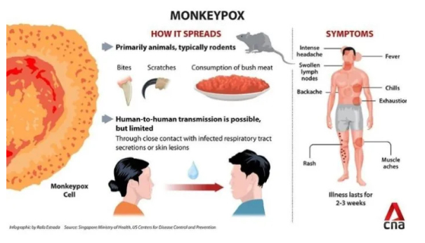
Research article Special Issues

New numerical dynamics of the fractional monkeypox virus model transmission pertaining to nonsingular kernels

1.
Department of Mathematics, King Saud University, P. O. Box 22452, Riyadh 11495, Saudi Arabia
2.
Department of Mathematics, Saudi Electronic University, Riyadh, Saudi Arabia
3.
Department of Mathematics, Government College University, Faisalabad 38000, Pakistan
4.
Department of Mathematics, King Abdulaziz University, Jeddah, Saudi Arabia
5.
Department of Mathematics, Cankaya University, Ankara, Turkey
6.
Department of Medical Research, China Medical University Hospital, China Medical University, Taichung, Taiwan
7.
Department of Mathematics, SBK for Women University, Quetta, Pakistan

Academic Editor: Wandi Ding

Received: 03 July 2022 Revised: 22 September 2022 Accepted: 25 September 2022 Published: 09 October 2022

Monkeypox ( $\mathbb{MPX}$ ) is a zoonotic illness that is analogous to smallpox. Monkeypox infections have moved across the forests of Central Africa, where they were first discovered, to other parts of the world. It is transmitted by the monkeypox virus, which is a member of the Poxviridae species and belongs to the Orthopoxvirus genus. In this article, the monkeypox virus is investigated using a deterministic mathematical framework within the Atangana-Baleanu fractional derivative that depends on the generalized Mittag-Leffler (GML) kernel. The system's equilibrium conditions are investigated and examined for robustness. The global stability of the endemic equilibrium is addressed using Jacobian matrix techniques and the Routh-Hurwitz threshold. Furthermore, we also identify a criterion wherein the system's disease-free equilibrium is globally asymptotically stable. Also, we employ a new approach by combining the two-step Lagrange polynomial and the fundamental concept of fractional calculus. The numerical simulations for multiple fractional orders reveal that as the fractional order reduces from 1, the virus's transmission declines. The analysis results show that the proposed strategy is successful at reducing the number of occurrences in multiple groups. It is evident that the findings suggest that isolating affected people from the general community can assist in limiting the transmission of pathogens.

Keywords:

Monkeypox virus model,
Atangana-Baleanu differential operators,
existence-uniqueness,
qualitative analysis,
Lagrangre interpolating polynomial

Citation: Maysaa Al Qurashi, Saima Rashid, Ahmed M. Alshehri, Fahd Jarad, Farhat Safdar. New numerical dynamics of the fractional monkeypox virus model transmission pertaining to nonsingular kernels[J]. Mathematical Biosciences and Engineering, 2023, 20(1): 402-436. doi: 10.3934/mbe.2023019

Related Papers:

[1]	Zhongdi Cen, Jian Huang, Aimin Xu . A posteriori mesh method for a system of singularly perturbed initial value problems. AIMS Mathematics, 2022, 7(9): 16719-16732. doi: 10.3934/math.2022917
[2]	Lin Fan, Shunchu Li, Dongfeng Shao, Xueqian Fu, Pan Liu, Qinmin Gui . Elastic transformation method for solving the initial value problem of variable coefficient nonlinear ordinary differential equations. AIMS Mathematics, 2022, 7(7): 11972-11991. doi: 10.3934/math.2022667
[3]	Shuqin Zhang, Jie Wang, Lei Hu . On definition of solution of initial value problem for fractional differential equation of variable order. AIMS Mathematics, 2021, 6(7): 6845-6867. doi: 10.3934/math.2021401
[4]	Jean-Paul Chehab, Denys Dutykh . On time relaxed schemes and formulations for dispersive wave equations. AIMS Mathematics, 2019, 4(2): 254-278. doi: 10.3934/math.2019.2.254
[5]	Yu He, Jianing Yang, Theodore E. Simos, Charalampos Tsitouras . A novel class of Runge-Kutta-Nyström pairs sharing orders 8(6). AIMS Mathematics, 2024, 9(2): 4882-4895. doi: 10.3934/math.2024237
[6]	Jiadong Qiu, Danfu Han, Hao Zhou . A general conservative eighth-order compact finite difference scheme for the coupled Schrödinger-KdV equations. AIMS Mathematics, 2023, 8(5): 10596-10618. doi: 10.3934/math.2023538
[7]	Sara S. Alzaid, Pawan Kumar Shaw, Sunil Kumar . A numerical study of fractional population growth and nuclear decay model. AIMS Mathematics, 2022, 7(6): 11417-11442. doi: 10.3934/math.2022637
[8]	Daniel Clemente-López, Esteban Tlelo-Cuautle, Luis-Gerardo de la Fraga, José de Jesús Rangel-Magdaleno, Jesus Manuel Munoz-Pacheco . Poincaré maps for detecting chaos in fractional-order systems with hidden attractors for its Kaplan-Yorke dimension optimization. AIMS Mathematics, 2022, 7(4): 5871-5894. doi: 10.3934/math.2022326
[9]	Sen Ming, Xiaodong Wang, Xiongmei Fan, Xiao Wu . Blow-up of solutions for coupled wave equations with damping terms and derivative nonlinearities. AIMS Mathematics, 2024, 9(10): 26854-26876. doi: 10.3934/math.20241307
[10]	Huichol Choi, Kinam Sin, Sunae Pak, Kyongjin Sok, Sungryol So . Representation of solution of initial value problem for fuzzy linear multi-term fractional differential equation with continuous variable coefficient. AIMS Mathematics, 2019, 4(3): 613-625. doi: 10.3934/math.2019.3.613

Abstract

1. Introduction

We are exploring the initial value problem (IVP) defined as:

$\begin{equation} z^{\prime \prime } = f(t,z),\;z(t_{0}) = z_0,\;z^{\prime}(t_0) = z^{\prime}_0, \end{equation}$

(1.1)

where $f: \mathbb{R} \times \mathbb{R}^m\longrightarrow\mathbb{R}^m$ and $z_0, \; z^{\prime}_0\in \mathbb{R}^m$ . The above equation is widely applicable in various scientific and engineering contexts. Notably, Eq (1.1) lacks $z^{\prime }$ .

The Numerov method facilitates the numerical advancement of the solution from $t_k$ to $t_{k+1} = h+t_k$ , a well-established approach for solving Eq (1.1). It is expressed as:

$z_{k+1} = 2z_k-z_{k-1}+\frac{h^2}{12}\left(f_{k+1}+10f_k+f_{k-1}\right),$

where $z_k\approx z(t_k)$ and $f_k\approx z^{\prime \prime }_n = f(t_k, z_k)$ . Note that $f_k, z_k\in\mathbb{R}^m$ .

Hairer ^[1], Cash ^[2] and Chawla ^[3] introduced hybrid implicit Numerov-type methods (i.e., using non-mesh points) approximately 40–45 years ago. Addressing the P-stability property, crucial for handling stiff oscillatory problems, was the primary challenge then. Chawla ^[4] proposed the modified Numerov scheme, evaluated explicitly as follows:

$\begin{equation} \begin{array}{c} v_1 = z_{k-1}, \\ v_2 = z_k, \\ v_3 = 2z_k-z_{k-1}+h^2f(t_k,v_2), \\ z_{k+1}-2z_k+z_{k-1} = \frac{1}{12}h^2\cdot (f(t_{k+1},v_3)+10f(t_k,v_2)+f(t_{k-1},v_1)), \\ \end{array} \end{equation}$

(1.2)

where $h$ is a constant step length:

$h = t_{k}-t_{k-1} = t_{k+1}-t_{k} = \cdots = t_1-t_0.$

The vectors $z_{k+1}, \; z_k$ , and $z_{k-1}$ approximate $z(t_k+h), \; z(t_k)$ , and $z(t_k-h)$ respectively, while $v_1\in\mathbb{R}^m, \; v_2\in\mathbb{R}^m$ , and $v_3\in\mathbb{R}^m$ represent the stages (alternatively named: function evaluations) used by the method.

We utilize the information known at the mesh:

$v_1 = z_{k-1},\:v_2 = z_k.$

Since $f(t_{k-1}, v_1)$ is computed in the previous step, only $f(t_{k+1}, v_3)$ and $f(t_{k}, v_2)$ need evaluation each step, resulting in only two function evaluations per step.

Tsitouras then introduced a Runge–Kutta–Nyström (RKN)-style method ^[5], significantly reducing the cost. Consequently, only four steps are required to create a sixth-order method, whereas previous implementations required six function evaluations (see ^[6]).

Subsequent to this, our group extensively investigated the topic. Tsitouras developed eighth-order methods with nine steps per step in ^[7]. Ninth-order methods were studied in ^[8]. Concurrently, a group of Spanish researchers conducted highly interesting work on the same topic ^[9,10,11].

In this study, we aim to present a new method for better addressing problems with periodic solutions. Traditionally, various properties from a simple test equation are fulfilled for this purpose. The novelty lies in training the available free parameters across a wide set of relevant problems. Differential evolution is employed for this training. It is anticipated that this methodology will yield a method better tuned for oscillatory problems.

2. Order conditions for hybrid Numerov-type methods

For the numerical treatment of Eq (1.1) with higher-order algebraic methods, there exists a considerable demand. We can represent the independent variable $t$ as one of the components of $z$ (if necessary, add $t^{\prime\prime} = 0$ see [, pg. 286] for details). Consequently, our focus, without loss of generality, lies on the autonomous system $z^{\prime\prime} = f(z)$ . Subsequently, a hybrid Numerov method with $s$ stages, as delineated in ^[7], may be expressed as:

$\begin{equation} \begin{array}{c} z_{k+1} = 2z_{k}-z_{k-1}+h^2\cdot \left( w\otimes I_{s}\right) \cdot f\left( v\right) ,\,\ v = \left( \textbf{1}+a\right) \otimes z_{k}-a\otimes z_{k-1}+ h^2\cdot \left( D\otimes I_{s}\right) \cdot f\left( v\right) \end{array} \end{equation}$

(2.1)

where $I_s \in \mathbb{R}^{s \times s}$ represents the identity matrix, $D \in \mathbb{R}^{s\times s}, w^T \in \mathbb{R}^s, a\; \in \mathbb{R}^s$ denote the coefficient matrices of the method, and

$\textbf{1} = [1\; 1\; \cdots 1]^T \in \mathbb{R}^s.$

To present the coefficients, we utilize the Butcher tableau ^[13,14],

$\begin{array}{c|c} a & D \\ \hline & w \end{array}.$

The method described in (1.2) can be represented using matrices ^[8]. As the function evaluations are computed sequentially, these methods are explicit. Therefore, $D$ represents a strictly lower triangular matrix. For the case when $s = 8$ , the method takes the following structure:

$\begin{eqnarray*} f_{k-1} & = &f\left( t_{k-1},z_{k-1}\right) \\ f_{k} & = &f\left( t_{k},z_{k}\right) \\ z_{\alpha} & = &a_{3}z_{k-1}+\left( 1-a_{3}\right) z_{k}+h^{2}\left(d_{31}f_{k-1}+a_{d2}f_{k}\right) ,\ \\ f_{\alpha} & = &f\left( t_{k}-a_{3}h,z_{\alpha}\right) , \\ z_{\beta} & = &a_{4}z_{k-1}+\left( 1-a_{4}\right) z_{k}+h^{2}\left(d_{41}f_{k-1}+d_{42}f_{k}+d_{43}f_{\alpha}\right) , \\ f_{\beta} & = &f\left( t_{k}-a_{4}h,z_{\beta}\right) , \\ z_{c} & = &a_{5}z_{k-1}+\left( 1-a_{5}\right) z_{k}+h^{2}\left(d_{51}f_{k-1}+d_{52}f_{k}+d_{53}f_{\alpha}+d_{54}f_{\beta}\right) , \\ f_{c} & = &f\left( t_{k}-a_{5}h,z_{c}\right) , \\ z_{\delta} & = &a_{6}z_{k-1}+\left( 1-a_{6}\right) z_{k}+h^{2}\left(d_{61}f_{k-1}+d_{62}f_{k}+d_{63}f_{\alpha}+d_{64}f_{\beta}+d_{65}f_{c}\right) , \\ f_{\delta} & = &f\left( t_{k}-a_{6}h,z_{\delta}\right) , \\ z_{e} & = &a_{7}z_{k-1}+\left( 1-a_{7}\right) z_{k}+h^{2}\left(d_{71}f_{k-1}+d_{72}f_{k}+d_{73}f_{\alpha}+d_{74}f_{\beta}+d_{75}f_{c}+d_{76}f_{\delta} \right) , \\ f_{e} & = &f\left( t_{k}-a_{7}h,z_{e}\right) , \\ z_{g} & = &a_{8}z_{k-1}+\left( 1-a_{8}\right) z_{k}+h^{2}\left( d_{81}f_{k-1}+d_{82}f_{k}+d_{83}f_{\alpha}+d_{84}f_{\beta}+d_{85}f_{c}+d_{86}f_{\delta}+d_{87}f_{e}\right) , \\ z_{k+1} & = &2z_{k}-z_{k-1}+h^{2}\left( w_{1}f_{k-1}+w_{2}f_{k}+w_{3}f_{\alpha}+w_{4}f_{\beta}+w_{5}f_{c}+w_{6}f_{\delta}+w_{7}f_{e}+w_{8}f_{g}\right) . \end{eqnarray*}$

After assuming ^[15]

$w_3 = 0,w_5 = w_4,w_7 = w_6,w_8 = w_1,a_5 = -a_4,a_6 = -a_7,a_8 = 1,$

the associated matrices take the form

$\begin{equation*} D = \left[ \begin{array}{llllllll} 0 & 0 & 0 & 0 & 0 & 0 & 0 & 0 \\ 0 & 0 & 0 & 0 & 0 & 0 & 0 & 0 \\ d_{31} & d_{32} & 0 & 0 & 0 & 0 & 0 & 0 \\ d_{41} & d_{42} & d_{43} & 0 & 0 & 0 & 0 & 0 \\ d_{51} & d_{52} & d_{53} & d_{54} & 0 & 0 & 0 & 0 \\ d_{61} & d_{62} & d_{63} & d_{64} & d_{65} & 0 & 0 & 0 \\ d_{71} & d_{72} & d_{73} & d_{74} & d_{75} & d_{76} & 0 & 0 \\ d_{81} & d_{82} & d_{83} & d_{84} & d_{85} & d_{86} & d_{87} & 0 \end{array} \right] , \end{equation*}$

$w = \left[ \begin{array}{llllllll} w_1 & w_2 & 0 & w_4 & w_4 & w_6 & w_6 & w_1 \end{array} \right]\;{\rm and}\; a = \left[ \begin{array}{llllllll} -1 & 0 & a_3 & a_4 & -a_4 & -a_5 & a_5 & 1 \end{array} \right] ^T. \nonumber$

Given that $f_{k-1}$ is determined from the preceding stage, seven function assessments are performed per step. To achieve an algebraic order eight, it is imperative to nullify the corresponding error truncation components (refer to ^[16]).

Our technique encompasses a total of $34$ parameters. As noted earlier, there exist $27$ coefficients for matrix $D$ , denoted as

$d_{31}, d_{32}, d_{41}, d_{42}, d_{43}, \cdots , d_{87}.$

Moreover, there are $4$ coefficients associated with vector $w$ and $3$ elements pertaining to vector $a$ . The quantity of condition equations for various orders matches those of the RKN methods ^[17,18], as presented in . To attain an eighth order, a cumulative total of $1+1+2+3+6+10+20+36 = 79$ equations must be fulfilled. The equations up to the ninth order can be found in assorted tables within ^[16].

Table 1. Number of order conditions.

Order $p$	1	2	3	4	5	6	7	8	9	10	11
No of conditions	1	1	2	3	6	10	20	36	72	137	275

| Show Table

DownLoad: CSV

The parameters are fewer than the equations, presenting a comparable challenge encountered in devising Runge-Kutta (RK) techniques. Hence, we are compelled to employ simplifying assumptions that diminish the quantity of conditions, thereby also decreasing the number of coefficients. The most prevalent options include

$\begin{equation} \begin{array}{c} (D\cdot \textbf{1})_{(3-8)} = \frac 12\left( a^2+a\right)_{(3-8)} \\ (D\cdot a)_{(3-8)} = \frac 16\left( a^3-a\right)_{(3-8)} \\ (D\cdot a^2)_{(4-8)} = \frac {1}{12}\left( a^4+a\right)_{(4-8)} \end{array} \end{equation}$

(2.2)

with

$a^i = \left[ \begin{array}{llllllll} (-1)^i & 0 & a_3^i & a_4^i & (-a_4)^i & (-a_5)^i & a_5^i & 1\end{array} \right]^T,$

and for $\kappa_1 < \kappa_2$

$(v)_{(\kappa_1-\kappa_2)} = [v_{\kappa_1}\; v_{\kappa_1+1} \cdots v_{\kappa_2}]^T.$

The remaining order conditions are presented in Table 2. In this table, the symbol "*" can be interpreted as element-wise multiplication:

$[u_1\;\;u_2 \cdots u_n]^T*[v_1\;\;v_2 \cdots v_n]^T = [u_1 v_1\;\;u_2 v_2 \cdots u_n n_n]^T.$

Table 2. Equations of condition up to eighth order, under assumptions (2.2).

$w\cdot \textbf{1}=1,$ $w\cdot a^2=\frac16,$	$w\cdot a^4=\frac{1}{15},$	$w\cdot a^6=\frac{1}{28},$
$w\cdot D^{2}\cdot a=0,$	$w\cdot D^{3}\cdot \textbf{1}=\frac{1}{20160},$	$w\cdot D\cdot \left(a\ast D c\right) =-\frac{11}{15120},$
$w\cdot D^{3}\cdot a=0,$	$w\cdot D\cdot \left(a\ast D^{2}\cdot \textbf{1}\right) =\frac{1}{7560},$	$w\cdot \left(a\ast D^{2}c\right) =\frac{17}{10080},$
$w\cdot \left(a\ast D\cdot \left(a\ast D\cdot a\right) \right) =-\frac{1}{720},$	$w\cdot \left(a\ast D^{3}\cdot \textbf{1}\right) =\frac{23}{60480},$	$w\cdot \left(D\cdot \textbf{1}\ast D^{2}\cdot a\right) =\frac{17}{20160}.$

| Show Table

DownLoad: CSV

This operation holds lower precedence. Parentheses, exponents, and dot products are always computed prior to "*".

Given the thirteen order conditions outlined in and the fulfillment of $17$ assumptions (2.2), we determine that only thirty equations are necessary. This results in four coefficients remaining as variables. Let's consider $a_3, a_4, a_5$ , and $d_{64}$ . The issue can be resolved explicitly, and the corresponding efficient Mathematica ^[19] module is depicted in Table 3.

Table 3. Mathematica listing for the derivation of the coefficients with respect to

$a_3, a_4, a_5$ and

$d_{64}$ .

BeginPackage["Numerov8'"];

Clear["Numerov8'*"]

Numerov8::usage = " Numerov8[x1, x2, x3, x4] for 7-stages 8-order explicit Numerov"

Begin["'Private'"];

Clear["Numerov8'Private'*"];

Numerov8[aa3_?NumericQ, aa4_?NumericQ, aa5_?NumericQ, dd64_?NumericQ] :=

Module[{a3, a4, a5, w, w1, w2, w4, w6, w7, a, d, d31, d32, d41, d42, d43,

d85, d54, d61, d63, d72, d74, d53, d51, d84, d62, d52, e, so,

d87, d75, d64, d71, d81, d83, d85, d65, d73, d82, d86, d76},

w = {w1, w2, 0, w4, w4, w6, w6, w1};

a = {-1, 0, a3, a4, -a4, -a5, a5, 1};

d = {{0, 0, 0, 0, 0, 0, 0, 0},

{0, 0, 0, 0, 0, 0, 0, 0},

{d31, d32, 0, 0, 0, 0, 0, 0},

{d41, d42, d43, 0, 0, 0, 0, 0},

{d51, d52, d53, d54, 0, 0, 0, 0},

{d61, d62, d63, d64, d65, 0, 0, 0},

{d71, d72, d73, d74, d75, d76, 0, 0},

{d81, d82, d83, d84, d85, d86, d87, 0}};

e = {1, 1, 1, 1, 1, 1, 1, 1};

a3 = Rationalize[aa3, 10^-17]; a4 = Rationalize[aa4, 10^-17];

a5 = Rationalize[aa5, 10^-17]; d64 = Rationalize[dd64, 10^-17];

so = Solve[{-1 + w. e, -(1/12) + w. a^2/2, -(1/360) + w. a^4/24,

-(1/20160) + w. a^6/720} == {0, 0, 0, 0}, {w1, w2, w4, w6}];

w = Simplify[w /. so[[1]]];

so = Solve[

Join[(d. e - 1/2*(a^2 + a))[[3;; 8]], (d. a - 1/6*(a^3 - a))[[3;; 8]],

(d. a^2 - 1/12*(a^4 + a))[[4;; 8]], {w. d. d. a,

w. d. d. d. e - 1/20160, w. d. (a d. a) + 11/15120,

- w. d. d. d. a, w. d. (a d. d. e) + 1/7560,

w. (a d. d. a) - 17/10080, w. (a d. (a d. a)) + 1/720,

w. (a d. d. d. e) - 23/60480, w. (d. e d. d. a) - 17/20160}]

== Array[0 &, 26],

{d32, d31, d42, d41, d52, d51, d62, d61, d72, d71, d82, d81, d43,

d53, d63, d73, d83, d54, d65, d74, d75, d76, d84, d85, d86, d87}];

d = Simplify[d /. so][[1]];

Return[{a, w, d}]]

End[];

EndPackage[];

| Show Table

DownLoad: CSV

For comprehensive details regarding the computation of truncation error coefficients, refer to the comprehensive overview in ^[16]. Coleman ^[20] emphasized the utilization of the B2 series representation of the local truncation error, drawing connections with the T2 rooted trees.

3. Phase-lag and amplification errors

In ^[21], the scalar test problem

$\begin{equation} z^{\prime\prime } = -\omega ^2z,\; \; \omega \in \mathbb{R}, \end{equation}$

(3.1)

was introduced to examine the periodic characteristics of techniques applied to solve (1.1).

Upon employing a Numerov-style approach akin to (2.1) to tackle problem (3.1), a discrete equation is formulated, taking the form

$\begin{equation} z_{k+1}+S\left( \psi^2\right) z_{k}+P\left( \psi^2\right) z_{k-1} = 0, \end{equation}$

(3.2)

where $\psi = \omega h,$ and $S\left(\psi^2\right), P\left(\psi^2\right)$ represent polynomials in $\psi^2$ .

The periodicity interval $(0, \psi_0)$ encompasses all $0 < \psi < \psi_0$ with $P\left(\psi^2\right)\equiv 1$ and $0 < | S\left(\psi^2\right) | < 2$ . A method deemed P-stable exhibits $\psi_0 = \infty$ .

The fulfillment of the zero dissipation property necessitates that

$P\left( \psi^2\right) = 1-\psi^2 w\left(I_s+\psi^2 D \right)^{-1} a\equiv 1,$

ensuring that the numerical method approximating (3.1) remains within its cyclic orbit.

The dissipation order $\rho$ of a method is characterized by the number for which $1-P\left(\psi^2\right) = O(\psi^{\rho})$ . It is worth noting that

$P\left( \psi^2\right) = 1+\sum\limits_{j = 0}^\infty \psi^{2j+1} w \cdot D^j \cdot a = 1+\psi q_1+\psi^3 q_3+\cdots.$

A method with algebraic order $2 \cdot i$ satisfies the terms in the aforementioned series for $j = 0, 1, \cdots, i-1$ . Consequently, for an eighth order method, it is advantageous to address

$q_9 = w \cdot D^4 \cdot a = 0, \; q_{11} = w \cdot D^5 \cdot a = 0, \cdots \; \; \mbox{etc.},$

to enhance the dissipation order. In the case of a zero-dissipative method, only $q_9 = z_{11} = q_{13} = q_{15} = q_{17} = 0$ is necessary, and as for the lower triangular matrix $D$ , all other $q'$ -s vanish,

$q_{2i+1} = w \cdot D^i \cdot a = 0, \; \mbox{for} \; i > 8.$

The difference in angles between the numerical and theoretical cyclic solution of (3.1) is called phase-lag. Since the solution of (3.1) is

$z(t) = e^{\omega t\sqrt{-1}},$

we may write Eq (3.2) as

$\begin{equation} \Lambda = e^{2\psi\sqrt{-1}}+S\left( \psi^2\right) \cdot e^{\psi\sqrt{-1}}+P\left( \psi^2\right) = O(\psi^{\tau}), \end{equation}$

(3.3)

with the number $\tau$ the phase-lag order of the method. Since

$S\left( \psi^{2} \right) = 2-\psi^2 w \cdot \left(I+\psi^2 D \right)^{-1} \cdot \left( \textbf{1}+a \right),$

we observe that expression (3.3) is a series of the form

$\begin{equation} \Lambda = \sum\limits_{i = 1}^\infty \psi^{2i} (-1)^{i+1} \left( \sum\limits_{j = 1}^{i} \frac 1{(2(i-j))!} w \cdot D^{j-1} \cdot \left( \textbf{1} + a \right) - w \cdot D^{i-1} \cdot a - 2 \sum\limits_{j = 1}^i \frac {1}{(2j)! \cdot (2(i-j))!} \right), \end{equation}$

(3.4)

or in a compact form

$\Lambda = \psi^2 \lambda_2+\psi^4 \lambda_4+\psi^6 \lambda_6+O(\psi^{8}).$

In this series, $\lambda_2 = \lambda_4 = \cdots = \lambda_{2i} = 0$ for $i = 1, 2, \cdots, \lfloor \frac{p-1}{2} \rfloor+1$ , where $p$ denotes the algebraic order of the method. For eighth order methods, the order conditions yield $\lambda_2 = \lambda_4 = \lambda_6 = \lambda_8 = 0$ . Given that $p = 8$ , and for $i = 3$ , we infer from (3.4):

$\lambda_6 = \frac{1}{(2\cdot(3-1))!}w\cdot( \textbf{1}+a)+\frac{1}{2!}w\cdot D\cdot( \textbf{1}+a)+w\cdot D^2\cdot \textbf{1}-2\cdot(\frac{1}{2!4!}+\frac{1}{4!2!}+\frac{1}{6!0!}) = 0.$

In case of $i = 4$ , we get (observe already that $w\cdot \textbf{1} = 1, \; w\cdot c = 0, \; w\cdot D\cdot c = 0,$ etc.),

$\lambda_8 = -\frac{127}{20160}+\frac{1}{720} (w\cdot a+w\cdot \textbf{1})+\frac{1}{24}(w\cdot D\cdot a+w\cdot D\cdot \textbf{1})$

$+\frac{1}{2}(w\cdot D^2\cdot a +w\cdot D^2 \cdot \textbf{1})+w\cdot D^3\cdot \textbf{1} = 0.$

Further we have that,

$\lambda_{10} = w\cdot D^4\cdot \textbf{1}-\frac{1}{1814400},$

$\lambda_{12} = \frac12w\cdot D^4\cdot a+w\cdot D^5\cdot \textbf{1}-\frac{1}{239500800},$

$\lambda_{14} = \frac{1}{24} w\cdot D^4\cdot c+\frac{1}{2} w\cdot D^5\cdot a+\frac{1}{2} w\cdot D^5\cdot \textbf{1}+w\cdot D^6\cdot \textbf{1}-\frac{23}{10897286400},$

$\lambda_{16} = \frac{1}{720} w\cdot D^4\cdot c+\frac{1}{24} w\cdot d^5\cdot c+\frac{1}{24} w\cdot D^5\cdot \textbf{1}$

$\; \; \; \; \; \; \; \; \; \; \; \; \; \; \; \; \; \; \; \; \; \; \; \; \; \; \; \; \; \; +\frac{1}{2}w\cdot D^6\cdot c+\frac{1}{2} w\cdot D^6\cdot \textbf{1}+w\cdot D^7\cdot \textbf{1}-\frac{647}{3487131648000}.$

Then we may ask for simultaneous satisfaction of phase-lag order conditions:

$\begin{equation} \lambda_{10} = 0, \; \lambda_{12} = 0, \; \lambda_{14} = 0, \; \lambda_{16} = 0. \end{equation}$

(3.5)

The set of four nonlinear equations (3.5) can be resolved to determine the four independent parameters. Our analysis reveals that the method exhibits a phase error on the order of $O(\psi^{18})$ , whereas the amplification error is $O(\psi^{9})$ . Consequently, the newly devised method demonstrates dissipative characteristics and lacks a periodicity interval.

The free parameters satisfying (3.5) in double precision are the following ^[15],

$a_3 = 0.870495922977052833,\:a_4 = -0.265579060733883584,$

$a_5 = -1.11694341482497459,\:d_{64} = -2.43624015403357971,$

and form the method N8ph18 that outperforms other methods in oscillatory problems.

Another noteworthy characteristic is P-stability ^[2,3]. In this context, it is essential to ensure $\sigma\equiv1$ , while also meeting the condition

$-2\leq(2-\psi^2w\cdot(I_s-\psi^2D)^{-1}\cdot( \textbf{1}+a))\leq2.$

Only implicit methods are capable of fulfilling these two criteria simultaneously.

4. Training the free parameters in a wide set of periodic problems

From the aforementioned set, our aim is to create a specific hybrid Numerov-style approach. The resultant technique should excel when applied to challenges exhibiting oscillatory solutions. Therefore, we opt to evaluate the following scenarios for testing purposes.

$z^{\prime \prime }(x) = -\mu ^{2}z(t),\;z(0) = 1,z^{\prime }(0) = 0,t\in \lbrack 0,10\pi],$

with the analytical solution $z(t) = \cos (\mu x)$ . This scenario was tested using five distinct values of $\mu$ : specifically, $\mu = 1, 3, 5, 7, 9.$ These numbers were chosen arbitrarily. Different choices will produce slightly different coefficients. Anyway, Differential Evolution is a metaheuristic method that produces random results in (hopefully) the direction of desired solutions. We may get thousands of results extremely close to each other. Consequently, we have five scenarios denoted as 1–5.

Our current project's primary framework is rooted in ^[22]. Upon selection of the independent parameters $a_3, a_4, a_5, d_{64}$ , we establish a method termed NEW8. Each scenario undergoes four runs with varying step counts. For each run we evaluated the maximum global error $ge_{\rm problem, steps}$ observed and we record the "accurate digits" i.e., $-log_{10}{(ge_{\rm problem, steps})}$ . The mean value $r$ , computed over these 20 problems, serves as an efficacy metric to be optimized. To facilitate this optimization, we employ the differential evolution technique ^[23].

DE operates through iterative steps, where each iteration, or generation $g$ , involves a "population" of individuals $\left(a_{3, i}^{(g)}, a_{4, i}^{(g)}, a_{5, i}^{(g)}, d_{64, i}^{(g)}\right)$ , $i = 1, 2, \cdots, N$ , with $N$ denoting the population size. The initial population $\left(a_{3, i}^{(0)}, a_{4, i}^{(0)}, a_{5, i}^{(0)}, d_{64, i}^{(0)}\right)$ , $i = 1, 2, \cdots, N$ is randomly generated in the first step. Furthermore, we designate $r$ as the fitness function, computed as the average precision over the 20 aforementioned runs. This fitness function is then assessed for each individual within the initial population. In every generation (iteration) $g$ , a three-step sequential process updates all individuals involved, consisting of Differentiation, Crossover, and Selection.

We utilized MATLAB ^[24] software DeMat ^[25] for the implementation of the aforementioned technique. Indeed, notable enhancements were achieved through selection:

$\begin{array}{ll} a_3 = 0.9442042052877105, & a_4 = 0.4611624530665672, \\ a_5 = -0.8575664014828354, & d_{64} = 12.56127525577038 . \end{array}$

The coefficients of the new method in matrix forms are given below, which are suitable for double precision computations.

$D = \left( \begin{array}{cccccccc} 0 & 0 & 0 & 0 & 0 & 0 & 0 & 0 \\ 0 & 0 & 0 & 0 & 0 & 0 & 0 & 0 \\ \frac{13073231}{765816835} & \frac{1162425931}{1290448873} & 0 & 0 & 0 & 0 & 0 & 0 \\ \frac{15504301}{303446304} & \frac{204546529}{691503620} & -\frac{5468561}{548112870} & 0 & 0 & 0 & 0 & 0 \\ -\frac{46437667}{980424298} & -\frac{95091815}{1054858556} & \frac{13784899}{946911356} & -\frac{1290636}{998791667} & 0 & 0 & 0 & 0 \\ -\frac{2384643161}{951946033} & -\frac{5551854734}{301857693} & -\frac{862090392}{293777917} & \frac{897911057}{71482476} & \frac{10304258074}{853918619} & 0 & 0 & 0 \\ \frac{276746015}{1037399899} & \frac{1131050235}{688407688} & \frac{186740362}{1030099325} & -\frac{1139314213}{1212843869} & -\frac{1500147825}{1231327489} & \frac{6071398}{1089814211} & 0 & 0 \\ -\frac{34899406663}{1129559599} & -\frac{291110149698}{1237155877} & -\frac{44963114191}{1183071678} & \frac{62726461355}{397241959} & \frac{142749796241}{969555741} & \frac{123970163}{1671884409} & -\frac{1993137}{584124064} & 0 \\ \end{array} \right),\nonumber$

$w = \left[ \begin{array}{cccccccc} -\frac{1341579}{392312827} & \frac{461160043}{1084958442} & 0 & \frac{306071289}{1258074655} & \frac{306071289}{1258074655} & \frac{42607879}{894937316} & \frac{42607879}{894937316} & -\frac{1341579}{392312827} \end{array} \right],\nonumber$

and

$a = \left[ \begin{array}{cccccccc} -1 & 0 & \frac{198781151}{210527712} & \frac{43361502}{94026523} & -\frac{43361502}{94026523} & \frac{96673439}{112729975} & -\frac{96673439}{112729975} & 1 \end{array} \right] ^T. \nonumber$

With this approach, we achieved a value of approximately $r\approx9.24$ , which demonstrates remarkable performance. In fact, numerous methods yielding $r > 9.1$ were obtained, indicating the presence of a narrow range of parameter combinations $a_3, a_4, a_5, d_{64}$ where $r$ reaches elevated levels. It is noteworthy that in the current configuration, the amplification differs from unity ( $\sigma\neq1$ ), and the phase lag is on the order of $O(v^8)$ , implying $\rho = O(v^8)$ , where $\rho_8\neq0$ . Moreover, no specific property is satisfied under these conditions.

In we present the results for the new method and the method N8ph18 presented in ^[15] that was especially formed for addressing oscillatory problems. For this latter method we observe a performance $\rho\approx7.82$ which is much smaller.

Table 4. Training phase. Accurate digits delivered after using various steps by NEW

$8$ and N

$8$ ph18 in the interval

$[0, 10\pi]$ .

Problem	Steps	NEW8	N8ph18
$1$	$20$	$7.5$	$6.6$
	$40$	$11.2$	$9.4$
	$60$	$12.3$	$11.0$
	$80$	$13.3$	$12.1$
$2$	$50$	$6.0$	$5.4$
	$100$	$10.1$	$8.2$
	$150$	$11.2$	$9.8$
	$200$	$12.0$	$10.9$
$3$	$80$	$5.6$	$5.0$
	$130$	$8.2$	$7.0$
	$180$	$10.8$	$8.3$
	$230$	$12.0$	$9.2$
$4$	$100$	$4.7$	$4.4$
	$150$	$7.0$	$6.0$
	$200$	$8.6$	$7.2$
	$250$	$11.0$	$8.1$
$5$	$150$	$5.5$	$4.9$
	$225$	$7.7$	$6.6$
	$300$	$9.6$	$7.7$
	$375$	$10.3$	$8.6$

| Show Table

DownLoad: CSV

5. Numerical results

The NEW8 method was designed to excel following multiple iterations on model scenarios. In the assessments outlined in Table 4, it was anticipated to outperform alternative methods for the specified intervals and step counts.

Hence, we aim to subject NEW8 to a distinct array of challenges, encompassing varying intervals and step counts. To this end, we re-evaluate problems 1–5 over an extended interval $[0, 20\pi]$ . These problems are now labeled as $1^{\prime}, 2^{\prime}, \cdots, 5^{\prime}$ . Additionally, we introduce two additional nonlinear problems and a wave equation to broaden the scope of evaluation. Specifically, we consider:

5.1. The inhomogeneous problem

$z^{\prime \prime }(t) = -100z(t)+99\sin t,\;z(0) = 1,z^{\prime }(0) = 11,t\in \lbrack0,20\pi ],$

with the theoretical solution $z(t) = \cos (10t)+\sin (10t)+\sin t$ .

5.2. The Duffing equation

Next, we choose the equation

$\begin{eqnarray*} z^{\prime \prime }(t) & = &\frac{1}{500}\cdot \cos \left( 1.01t\right) -z(t)-z(t)^{3}, \\ z(0) & = &0.2004267280699011,z^{\prime }\left( 0\right) = 0, \end{eqnarray*}$

with an approximate analytical solution given in ^[16],

$\begin{equation*} z(t)\approx \left\{ \begin{array}{l} 6\cdot 10^{-16}\cos (11.11t)+4.609\cdot 10^{-13}\cos (9.09t) \\ +3.743495\cdot 10^{-10}\cos (7.07t)+3.040149839\cdot 10^{-7}\cos (5.05t) \\ +2.469461432611\cdot 10^{-4}\cos (3.03t)+0.2001794775368452\cos (1.01t) \end{array} \right\}. \end{equation*}$

5.3. Wave equation

Finally, we consider the linearized wave equation, which is a rather large-scale problem ^[16],

$\begin{eqnarray*} \frac{\vartheta ^2u}{\vartheta t^2} & = &4\frac{\vartheta ^2u}{\vartheta x^2} +\sin t\cdot \cos \left( \frac{\pi x}b\right) ,\ 0\leq x\leq b = 100,\ t\in [0,20\pi ], \\ \frac{\vartheta u}{\vartheta x}\left( t,0\right) & = &\frac{\vartheta u}{ \vartheta x}\left( t,b\right) = 0, \\ u\left( 0,x\right) &\equiv &0,\ \frac{\vartheta u}{\vartheta t}\left( 0,x\right) = \frac{b^2}{4\pi ^2-b^2}\cos \frac{\pi x}b, \end{eqnarray*}$

with the theoretical solution

$\begin{equation} u\left( t,x\right) = \frac{b^2}{4\pi ^2-b^2}\cdot \sin t\cdot \cos \frac{\pi x }b. \end{equation}$

(5.1)

We discretize $\frac{\vartheta ^2u}{\vartheta x^2}$ using fourth-order symmetric differences for internal points, while boundary points utilize one-sided differences of the same order (while considering the information about $\frac{\vartheta u}{\vartheta x}$ at those points). This results in the following system:

$\begin{eqnarray*} \left[ \begin{array}{l} z_0^{\prime \prime } \\ z_1^{\prime \prime } \\ \\ \\ z_N^{\prime \prime } \end{array} \right] & = &\frac 4{\left( \Delta x\right) ^2}\left[ \begin{array}{cccccccc} -\frac{415}{72} & 8 & -3 & {\frac 89} & -\frac 18 & & & \\ \frac{257}{144} & -\frac{10}3 & \frac74 & -\frac29 & \frac 1{48} & & 0 & \\ -\frac 1{12} & \frac 43 & -\frac 52 & \stackrel{}{\frac 43} & -\frac 1{12} & & & \\ & & \ddots & \ddots & \ddots & \ddots & \ddots & \\ & & & -\frac 1{12} & {\frac 43} & -\frac 52 & \frac 43 & -\frac 1{12} \\ & 0 & & \frac 1{48} & -\frac 29 & \frac74 & -\frac{10}3 & \frac{257}{144} \\ & & & -\frac 18 & \frac89 & -3 & 8 & -\frac{415}{72} \end{array} \right] \cdot \left[ \begin{array}{c} z_0 \\ z_1 \\ \vdots \\ \\ z_N \end{array} \right] \\ &&+\sin t\cdot \left[ \begin{array}{c} \cos \left( \frac{0\cdot \Delta x}b\cdot \pi \right) \\ \stackrel{}{\cos \left( \frac{1\cdot \Delta x}b\cdot \pi \right) } \\ \vdots \\ \\ \cos \left( \frac{N\cdot \Delta x}b\cdot \pi \right) \end{array} \right] . \end{eqnarray*}$

Here, $z_0, z_1\cdots z_N$ may be understood as coordinates of $z\in\mathbb{R}^{N+1}$ , and not as time steps. Upon selecting $\Delta x = 5$ , we establish a system with constant coefficients and $N = 20$ . The outcomes for this scenario were primarily influenced by the errors arising from the semi-discretization process. As a consequence, an error of about $10^{-6.1}$ is added constantly to the theoretical solution (5.1). Thus, no method can have a true error smaller than this. But, as shown in Table 5, our new method even though it has limited accuracy, is faster (i.e., uses fewer time steps) than N8ph18.

Table 5. Numerical tests phase. Accurate digits delivered after using various steps by NEW

$8$ and N

$8$ ph18 in the interval

$[0, 20\pi]$ .

Problem	Steps	NEW8	N8ph18
$1^{\prime}$	$40$	$7.2$	$6.3$
	$80$	$10.9$	$9.1$
	$120$	$12.0$	$10.7$
	$160$	$12.9$	$11.8$
$2^{\prime}$	$100$	$5.7$	$5.1$
	$200$	$9.8$	$7.9$
	$300$	$10.9$	$9.5$
	$400$	$11.7$	$10.6$
$3^{\prime}$	$160$	$5.2$	$4.7$
	$260$	$7.9$	$6.7$
	$360$	$10.5$	$8.0$
	$460$	$12.0$	$8.9$
$4^{\prime}$	$200$	$4.4$	$4.1$
	$300$	$6.7$	$5.7$
	$400$	$8.3$	$6.9$
	$500$	$10.7$	$7.8$
$5^{\prime}$	$300$	$5.2$	$4.6$
	$450$	$7.4$	$6.2$
	$600$	$9.3$	$7.4$
	$750$	$10.0$	$8.3$
$6$	$240$	$2.9$	$3.0$
	$480$	$7.0$	$5.9$
	$720$	$10.1$	$7.5$
	$960$	$10.1$	$8.6$
$7$	$100$	$4.8$	$4.9$
	$200$	$7.7$	$7.3$
	$300$	$9.3$	$8.7$
	$400$	$10.4$	$9.7$
$8$	$60$	$6.0$	$5.0$
	$70$	$6.1$	$5.4$
	$80$	$6.1$	$5.8$
	$90$	$6.1$	$5.9$

| Show Table

DownLoad: CSV

We execute these $8$ scenarios with varying step counts and present the outcomes in Table 5. Notably, we also incorporate results obtained using the N8ph18 method. For economy and ease of reading the results, only the best methods of eighth order were tested on oscillatory problems. i.e., NEW8 and N8ph18. N8ph18 has already proven to outperform other 8th order methods ^[15,16]. It becomes evident from the table that NEW8 significantly outperforms all other methods documented in the literature. Overall, an improvement of nearly one decimal digit in accuracy was achieved.

The proposed method is constructed for application to second order Ordinary Differential Equations (ODEs) with oscillatory solutions. However, this is a rather wide category of problems that is constantly under the interest of respected scholars. As seen from problem 8 (wave equation), our method may also apply to a certain kind of partial differential equations sharing periodic solutions after proper transformation to system of ODEs.

6. Conclusions

The key aspects of our investigation were as follows:

● We explored a family of eighth-order hybrid two-step techniques characterized by minimal stage counts, with a notable innovation being the proposal of a methodology for selecting appropriate independent parameters.

● The parameters of the novel technique were determined following extensive evaluation of their performance across a diverse array of periodic scenarios.

● Optimal parameter selection was achieved through the application of the differential evolution approach. Across a broad spectrum of challenges featuring oscillatory solutions, the devised approach demonstrated significant superiority over methods belonging to both similar and disparate families.

● The method we introduced is finely calibrated for scenarios with periodic solutions, particularly those featuring substantial linear components.

Author contributions

Both authors of this article have been contributed equally. Both authors have read and approved the final version of the manuscript for publication.

Use of AI tools declaration

The authors declare that no Artificial Intelligence (AI) tools were used in the creation of this article.

Conflict of interest

This work does not have any conflicts of interest.

References

[1]	A. W. Rimoin, P. M. Mulembakani, S. C. Johnstonm, J. O. Lloyd Smith, N. K. Kisalu, T. L. Kinkela, et al., Major increase in human monkeypox incidence 30 years after smallpox vaccination campaigns cease in the Democratic Republic of Congo, Proc. Natl. Acad. Sci. USA, 107 (2010), 16262–16267. http://dx.doi.org/10.1073/pnas.1005769107 doi: 10.1073/pnas.1005769107
[2]	N. Sklenovská, M. Van Ranst, Emergence of monkeypox as the most important orthopoxvirus infection in humans, Front. Public Health, 241 (2018). https://doi.org/10.3389/fpubh.2018.00241
[3]	Singapore Ministry of Health, Europe, US on alert over detection of Monkeypox cases: What is the virus, symptoms and its transmission across the globe. Available from: https://news.knowledia.com/IN/en/articles/europe-us-on-alert-over-detection-of-monkeypox-cases-what-is-the-virus-5.
[4]	F. Fenner, D. A. Henderson, I. Arita, Z. Jezek, I. D. Ladnyi, Smallpox and its eradication, W. H. O., 1988.
[5]	R. B. Kennedy, J. M. Lane, D. A. Henderson, G. A. Poland, Smallpox and vaccinia, Vaccines (chapter 32), Amsterdam: Elsevier, (2012), 718–727.
[6]	P. E. M. Fine, Z. Jezek, B. Grab, H. Dixon, The transmission potential of monkeypox virus in human populations, Int. J. Epidemiol. , 17 (1988), 643–650. http://dx.doi.org/10.1093/ije/17.3.643 doi: 10.1093/ije/17.3.643
[7]	K. D. Reed, J. W. Melski, M. B. Graham, R. L. Regnery, M. J. Sotir, M. V. Wegner, et al., The detection of monkeypox in humans in the Western Hemisphere, Engl. J. Med. , 350 (2004), 342–350. http://dx.doi.org/10.1056/ NEJMoa032299 doi: 10.1056/NEJMoa032299
[8]	M. Roberts, Monkeypox to get a new name, says WHO. Available from: https://en.kataeb.org/articles/monkeypox-to-get-a-new-name-says-who.
[9]	L. A. Learned, M. G. Reynolds, D. W. Wassa, Y. Li, V. A. Olson, K. Karem, et al., Extended interhuman transmission of monkeypox in a hospital community in the Republic of the Congo, Am. J. Trop. Med. Hygiene, 73 (2005), 428–434. https://doi.org/10.4269/ajtmh.2005.73.428 doi: 10.4269/ajtmh.2005.73.428
[10]	R. A. Elderfield, S. J. Watson, A. Godlee, W. E. Adamson, C. I. Thompson, J. Dunning, M. Fernandez-Alonso, D. Blumenkrantz, T. Hussell, M. Zambon, Accumulation of human-adapting mutations during circulation of A (H1N1) pdm09 influenza virus in humans in the United Kingdom, J. Virol. , 88 (2014), 13269–13283. https://doi.org/10.1128/JVI.01636-14 doi: 10.1128/JVI.01636-14
[11]	N. C. Elde, S. J. Child, M. T. Eickbush, J. O. Kitzman, K. S. Rogers, J. Shendure, et al., Poxviruses deploy genomic accordions to adapt rapidly against host antiviral defenses, Cell, 150 (2012), 831–841. https://doi.org/10.1016/j.cell.2012.05.049 doi: 10.1016/j.cell.2012.05.049
[12]	R. J. Jackson, A. J. Ramsay, C. D. Christensen, S. Beaton, D. F. Hall, I. A. Ramshaw, Expression of mouse interleukin-4 by a recombinant ectromelia virus suppresses cytolytic lymphocyte responses and overcomes genetic resistance to mousepox. J. Virol. , 75 (2001), 1205–1210. https://doi.org/10.1128/JVI.75.3.1205-1210.2001 doi: 10.1128/JVI.75.3.1205-1210.2001
[13]	S. Bidari, E. E. Goldwyn, Stochastic models of influenza outbreaks on a college campus, Lett. Biomath. , 6 (2019), 1–14. https://doi.org/10.1080/23737867.2019.1618744 doi: 10.1080/23737867.2019.1618744
[14]	J. C. Blackwood, L. M. Childs, An introduction to compartmental modeling for the budding infectious disease modeler. Lett. Biomath. , 5 (2018), 195–221. https://doi.org/10.30707/LiB5.1Blackwood doi: 10.30707/LiB5.1Blackwood
[15]	C. Bhunu, S. Mushayabasa, Modelling the transmission dynamics of Pox-like infections, IAENG Int. J. Appl. Math. , 41 (2011), 141–149.
[16]	S. Usman, I. I. Adamu, Modeling the transmission dynamics of the monkeypox virus infection with treatment and vaccination interventions, J. Appl. Math. Phy. , 5 (2017), 2335–2353. https://doi.org/10.4236/jamp.2017.512191 doi: 10.4236/jamp.2017.512191
[17]	A. Atangana, D. Baleanu, New fractional derivatives with nonlocal and non-singular kernel: Theory and application to heat transfer model, Therm. Sci. , 20 (2016), 763–769. https://doi.org/10.2298/TSCI160111018A doi: 10.2298/TSCI160111018A
[18]	S. A. Iqbal, M. G. Hafez, Y. M. Chu, C. Park, Dynamical Analysis of nonautonomous RLC circuit with the absence and presence of Atangana-Baleanu fractional derivative, J. Appl. Anal. Comput. 12 (2022), 770–789. https://doi.org/10.11948/20210324 doi: 10.11948/20210324
[19]	Y. M. Chu, S. Bashir, M. Ramzan, M. Y. Malik, Model-based comparative study of magnetohydrodynamics unsteady hybrid nanofluid flow between two infinite parallel plates with particle shape effects, Math. Meth. Appl. Sci., 2022. https://doi.org/10.1002/mma.8234
[20]	W. M. Qian, H. H. Chu, M. K. Wang, Y. M. Chu, Sharp inequalities for the Toader mean of order $-1$ in terms of other bivariate means, J. Math. Inequal. , 16 (2022), 127–141. https://doi.org/10.7153/jmi-2022-16-10 doi: 10.7153/jmi-2022-16-10
[21]	T. H. Zhao, H. H. Chu, Y. M. Chu, Optimal Lehmer mean bounds for the $n$ th power-type Toader mean of $n=-1, 1, 3$ , J. Math. Inequal. , 16 (2022), 157–168. https://doi.org/10.7153/jmi-2022-16-12 doi: 10.7153/jmi-2022-16-12
[22]	M. Caputo, M. Fabrizio, A new definition of fractional derivative without singular kernel, Progr. Fract. Differ. Appl. , 1 (2015), 1–13.
[23]	J. F. Gómez-Aguilar, H. Yéppez-Marténez, C. Calderón-Ramón, I. Cruz-Orduña, R. F. Escobar-Jiménez, V. H. Olivares-Peregrino, Modeling of a mass-spring-damper system by fractional derivatives with and without a singular kernel, Entropy, 17 (2015), 6289–6303. https://doi.org/10.3390/e17096289 doi: 10.3390/e17096289
[24]	F. Z. Wang, M. N. Khan, I. Ahmad, H. Ahmad, H. Abu-Zinadah, Y. M. Chu, Numerical solution of traveling waves in chemical kinetics: time-fractional fishers equations, Fractals, 30 (2022). https://doi.org/10.1142/S0218348X22400515
[25]	S. Rashid, E. I. Abouelmagd, S. Sultana, Y. M. Chu, New developments in weighted $n$ -fold type inequalities via discrete generalized ${\rm{\hat h}}$ -proportional fractional operators, Fractals, 30 (2022). https://doi.org/10.1142/S0218348X22400564
[26]	S. Rashid, B. Kanwal, A. G. Ahmad, E. Bonyah, S. K. Elagan, Novel numerical estimates of the pneumonia and meningitis epidemic model via the nonsingular kernel with optimal analysis, Complexity, 2022 (2022), 1–25. https://doi.org/10.1155/2022/4717663 doi: 10.1155/2022/4717663
[27]	S. W. Yao, S. Rashid, M. Inc, E. Elattar, On fuzzy numerical model dealing with the control of glucose in insulin therapies for diabetes via nonsingular kernel in the fuzzy sense, AIMS Math., 7 (2022). https://doi.org/10.3934/math.2022987
[28]	S. Rashid, F. Jarad, A. K. Alsharidi, Numerical investigation of fractional-order cholera epidemic model with transmission dynamics via fractal-fractional operator technique, Chaos Solitons Fractals, 162 (2022), 112477. https://doi.org/10.1016/j.chaos.2022.112477 doi: 10.1016/j.chaos.2022.112477
[29]	F. Jin, Z. S. Qian, Y. M. Chu, M. ur Rahman, On nonlinear evolution model for drinking behavior under Caputo-Fabrizio derivative, J. Appl. Anal. Comput. 12 (2022), 790–806. https://doi.org/10.11948/20210357 doi: 10.11948/20210357
[30]	S. Rashid, M. K. Iqbal, A. M. Alshehri, F. Jarad, R. Ashraf, A comprehensive analysis of the stochastic fractal-fractional tuberculosis model via Mittag-Leffler kernel and white noise, Results Phy. . 39 (2022), 105764. https://doi.org/10.1016/j.rinp.2022.105764 doi: 10.1016/j.rinp.2022.105764
[31]	M. Al-Qurashi, S. Rashid, F. Jarad, A computational study of a stochastic fractal-fractional hepatitis B virus infection incorporating delayed immune reactions via the exponential decay, Math. Biosci. Eng, 19 (2022), 12950–12980. https://doi.org/10.3934/mbe.2022605 doi: 10.3934/mbe.2022605
[32]	S. Rashid, A. Khalid, S. Sultana, F. Jarad, K. M. Abulanja, Y. S. Hamed, Novel numerical investigation of the fractional oncolytic effectiveness model with M1 virus via generalized fractional derivative with optimal criterion, Results Phy. , 37 (2022), 105553. https://doi.org/10.1016/j.rinp.2022.105553 doi: 10.1016/j.rinp.2022.105553
[33]	S. Rashid, B. Kanwal, F. Jarad, S. K. Elagan, A peculiar application of the fractal-fractional derivative in the dynamics of a nonlinear scabies model, Results Phys. , 38 (2022), 105634. https://doi.org/10.1016/j.rinp.2022.105634 doi: 10.1016/j.rinp.2022.105634
[34]	S. Rashid, Y. G. Sánchez, J. Singh, Kh. M. Abualnaja, Novel analysis of nonlinear dynamics of a fractional model for tuberculosis disease via the generalized Caputo fractional derivative operator (case study of Nigeria), AIMS Math. , 7 (2022), 10096–10121. https://doi.org/10.3934/math.2022562 doi: 10.3934/math.2022562
[35]	S. Rashid, F. Jarad, A. G. Ahmad, Kh. M. Abualnaja, New numerical dynamics of the heroin epidemic model using a fractional derivative with Mittag-Leffler kernel and consequences for control mechanisms, Results Phys. , 35 (2022), 105304. https://doi.org/10.1016/j.rinp.2022.105304 doi: 10.1016/j.rinp.2022.105304
[36]	S. N. Hajiseyedazizi, M. E. Samei, J. Alzabut, Y. M. Chu, On multi-step methods for singular fractional $q$ -integro-differential equations, Open Math. 19 (2021), 1378–1405. https://doi.org/10.1515/math-2021-0093 doi: 10.1515/math-2021-0093
[37]	S. Rashid, E. I. Abouelmagd, A. Khalid, F. B. Farooq, Y. M. Chu, Some recent developments on dynamical $\hbar$ -discrete fractional type inequalities in the frame of nonsingular and nonlocal kernels, Fractals, 30 (2022). https://doi.org/10.1142/S0218348X22401107
[38]	Y. M. Chu, U. Nazir, M. Sohail, M. M. Selim, J. R. Lee, Enhancement in thermal energy and solute particles using hybrid nanoparticles by engaging activation energy and chemical reaction over a parabolic surface via finite element approach, Fractal Fract. 5 (2021), 119. https://doi.org/10.3390/fractalfract5030119
[39]	T. Abdeljawad, D. Baleanu, Integration by parts and its applications of a new nonlocal fractional derivative with Mittag-Leffler nonsingular kernel, J. Nonlinear Sci. Appl. , 10 (2017), 1098–1107. http://dx.doi.org/10.22436/jnsa.010.03.20 doi: 10.22436/jnsa.010.03.20
[40]	J. Singh, D. Kumar, D. Baleanu, On the analysis of fractional diabetes model with exponential law, Adv. Differ. Equ. , 2018 (2018), 231. https://doi.org/10.1186/s13662-018-1680-1 doi: 10.1186/s13662-018-1680-1
[41]	Z. M. Odibat, N. T. Shawagfeh, Generalized Taylor's formula, Appl. Math. Comput. 186 (2007), 286–293. https://doi.org/10.1016/j.amc.2006.07.102 doi: 10.1016/j.amc.2006.07.102
[42]	S. V. Bankuru, S. Kossol, W. Hou, P. Mahmoudi, J. Rychtá ${\rm{\hat r}}$ , D. Taylor, A game-theoretic model of Monkeypox to assess vaccination strategies, PeerJ, 8 (2020), 9272. http://doi.org/10.7717/peerj.927 doi: 10.7717/peerj.927
[43]	O. J. Peter, S. Kumar, N. Kumari, F. A. Oguntolu, K. Oshinubi, R. Musa, Transmission dynamics of Monkeypox virus: A mathematical modelling approach, Model. Earth Sys. Envir., 2021. https://doi.org/10.1007/s40808-021-01313-2
[44]	M. Toufik, A. Atangana, New numerical approximation of fractional derivative with non-local and non-singular kernel: Application to chaotic models, Eur. Phys. J. Plus, 132 (2017), 444. https://doi.org/10.1140/epjp/i2017-11717-0 doi: 10.1140/epjp/i2017-11717-0
[45]	C. Bhunu, W. Garira, G. Magombedze, Mathematical analysis of a two strain hiv/aids model with antiretroviral treatment. Acta Biotheor. , 57 (2009), 361–381. https://doi.org/10.1007/s10441-009-9080-2 doi: 10.1007/s10441-009-9080-2
[46]	C. Bhunu, S. Mushayabasa, Modelling the transmission dynamics of pox-like infections, IAENG Int. J. Appl. Math. , 41 (2011), 141–149.
[47]	M. R. Odom, R. Curtis Hendrickson, E. J. Lefkowitz, Poxvirus protein evolution: Family wide assessment of possible horizontal gene transfer events, Virus Res. , 144 (2009), 233–249. https://doi.org/10.1016/j.virusres.2009.05.006 doi: 10.1016/j.virusres.2009.05.006
[48]	Y. Lia, Y. Chen, I. Podlubny, Mittag–Leffler stability of fractional order nonlinear dynamic systems, Automatica, 45 (2009), 1965–1969. https://doi.org/10.1016/j.automatica.2009.04.003 doi: 10.1016/j.automatica.2009.04.003
[49]	S. Somma, N. Akinwande, U. Chado, A mathematical model of monkey pox virus transmission dynamics, IFE J. Sci. , 21 (2019), 195–204. https://doi.org/10.4314/ijs.v21i1.17 doi: 10.4314/ijs.v21i1.17
[50]	O. Diekmann, J. Heesterbeek, M. G. Roberts, The construction of next-generation matrices for compartmental epidemic models, J. R. Soc. Interface, 7 (2010), 873–885. https://doi.org/10.1098/rsif.2009.0386 doi: 10.1098/rsif.2009.0386
[51]	P. van den Driessche, J. Watmough, Further notes on the basic reproduction number, Springer, Berlin, Heidelberg, (2008), 159–178.
[52]	C. Castillo-Chavez, B. Song, Dynamical models of tuberculosis and their applications, Math. Biosci. Eng. , 1 (2004), 361. https://doi.org/10.3934/mbe.2004.1.361 doi: 10.3934/mbe.2004.1.361
[53]	E. Ahmed, A. M. A. El-Sayed, H. A. A. El-Saka, On some routh–hurwitz conditions for fractional order differential equations and their applications in lorenz, rössler, chua and chen systems, Phys. Lett. A, 358 (2006), 1–4. https://doi.org/10.1016/j.physleta.2006.04.087 doi: 10.1016/j.physleta.2006.04.087
[54]	C. T. Deressa, G. F. Duressa, Analysis of Atangana–Baleanu fractional-order SEAIR epidemic model with optimal control, Adv. Diff. Equ. , 2021 (2021), 174. https://doi.org/10.1186/s13662-021-03334-8 doi: 10.1186/s13662-021-03334-8
[55]	B. Wu, F. Fu, L. Wang, Imperfect vaccine aggravates the long-standing dilemma of voluntary vaccination, PLOS ONE, 6 (2011), 20577. https://doi.org/10.1371/journal.pone.0020577 doi: 10.1371/journal.pone.0020577
[56]	L. Khodakevich, Z. Ježek, D. Messinger, Monkeypox virus: Ecology and public health significance, Bull. W. H. O. , 66 (1988), 747–752.
[57]	J. Kobe, N. Pritchard, Z. Short, I. V. Erovenko, J. Rychtář, J. T. Rowel, A game theoretic model of cholera with optimal personal protection strategies. Bull. Math. Bio., 80 (2018), 2580–2599. https://doi.org/10.1007/s11538-018-0476-5 doi: 10.1007/s11538-018-0476-5

Reader Comments

Your name:*

Email:*
© 2023 the Author(s), licensee AIMS Press. This is an open access article distributed under the terms of the Creative Commons Attribution License (http://creativecommons.org/licenses/by/4.0)