Driving factors and decoupling trend analysis between agricultural CO<sub>2</sub> emissions and economic development in China based on LMDI and Tapio decoupling

Jieqiong Yang; Panzhu Luo; Langping Li; Jieqiong Yang; Panzhu Luo; Langping Li

doi:10.3934/mbe.2022612

Mathematical Biosciences and Engineering

2022, Volume 19, Issue 12: 13093-13113. doi: 10.3934/mbe.2022612

Previous Article Next Article

Research article Special Issues

Driving factors and decoupling trend analysis between agricultural CO₂ emissions and economic development in China based on LMDI and Tapio decoupling

1.
College of Life Science and Technology, Central South University of Forestry and Technology, Changsha 410004, China
2.
College of Computer and Information Engineering, Central South University of Forestry and Technology, Changsha 410004, China

Received: 08 July 2022 Revised: 21 August 2022 Accepted: 29 August 2022 Published: 06 September 2022

Based on mathematical models, in-depth analysis about the interrelationship between agricultural CO₂ emission and economic development has increasingly become a hotly debated topic. By applying two mathematical models including logarithmic mean divisia index (LMDI) and Tapio decoupling, this work aims to study the driving factor and decoupling trend for Chinese agricultural CO₂ emission from 1996 to 2020. Firstly, the intergovernmental panel on climate change (IPCC) method is selected to estimate the agricultural CO₂ emission from 1996 to 2020, and the LMDI model is adopted to decompose the driving factors of agricultural CO₂ emission into four agricultural factors including economic development, carbon emission intensity, structure, and labor effect. Then, the Tapio decoupling model is applied to analyze the decoupling state and development trend between the development of agricultural economy and CO₂ emission. Finally, this paper puts forward some policies to formulate a feasible agricultural CO₂ emission reduction strategy. The main research conclusions are summarized as follows: 1) During the period from 1996 to 2020, China's agricultural CO₂ emission showed two stages, a rapid growth stage (1996–2015) and a rapid decline stage (2016–2020). 2) Agricultural economic development is the first driving factor for the increase of agricultural CO₂ emission, while agricultural labor factor and agricultural production efficiency factor play two key inhibitory roles. 3) From 1996 to 2020, on the whole, China's agricultural sector CO₂ emission and economic development showed a weak decoupling (WD) state. The decoupling states corresponding to each time period are strong negative decoupling (SND) (1996–2000), expansive negative decoupling (END) (2001–2005), WD (2006–2015) and strong decoupling (SD) (2016–2020), respectively.
- CO₂ emission,
- LMDI,
- decoupling analysis,
- China's agricultural sector
Citation: Jieqiong Yang, Panzhu Luo, Langping Li. Driving factors and decoupling trend analysis between agricultural CO2 emissions and economic development in China based on LMDI and Tapio decoupling[J]. Mathematical Biosciences and Engineering, 2022, 19(12): 13093-13113. doi: 10.3934/mbe.2022612

Related Papers:

Abstract

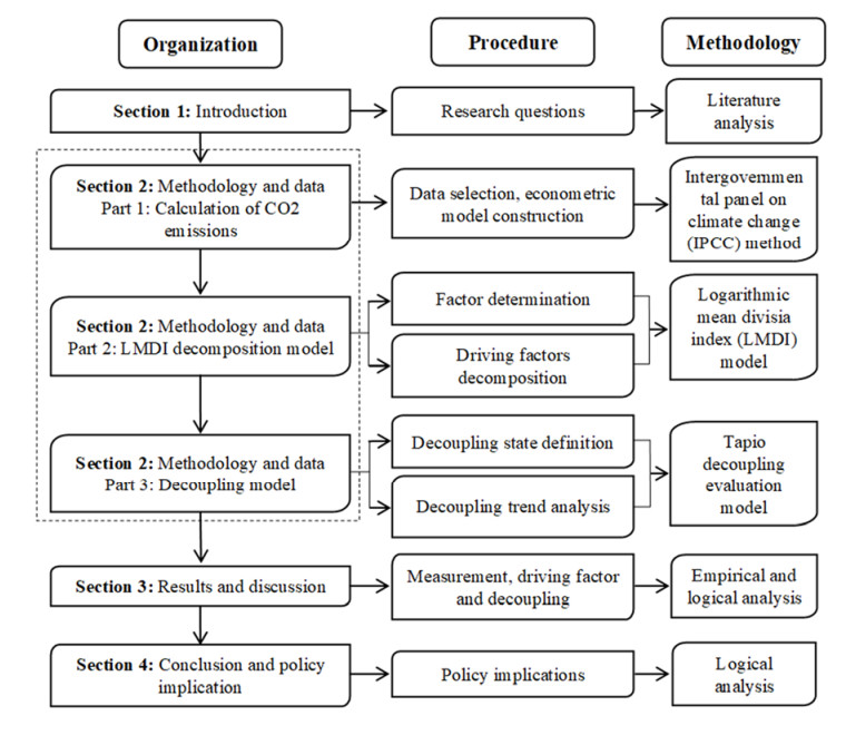
Based on mathematical models, in-depth analysis about the interrelationship between agricultural CO₂ emission and economic development has increasingly become a hotly debated topic. By applying two mathematical models including logarithmic mean divisia index (LMDI) and Tapio decoupling, this work aims to study the driving factor and decoupling trend for Chinese agricultural CO₂ emission from 1996 to 2020. Firstly, the intergovernmental panel on climate change (IPCC) method is selected to estimate the agricultural CO₂ emission from 1996 to 2020, and the LMDI model is adopted to decompose the driving factors of agricultural CO₂ emission into four agricultural factors including economic development, carbon emission intensity, structure, and labor effect. Then, the Tapio decoupling model is applied to analyze the decoupling state and development trend between the development of agricultural economy and CO₂ emission. Finally, this paper puts forward some policies to formulate a feasible agricultural CO₂ emission reduction strategy. The main research conclusions are summarized as follows: 1) During the period from 1996 to 2020, China's agricultural CO₂ emission showed two stages, a rapid growth stage (1996–2015) and a rapid decline stage (2016–2020). 2) Agricultural economic development is the first driving factor for the increase of agricultural CO₂ emission, while agricultural labor factor and agricultural production efficiency factor play two key inhibitory roles. 3) From 1996 to 2020, on the whole, China's agricultural sector CO₂ emission and economic development showed a weak decoupling (WD) state. The decoupling states corresponding to each time period are strong negative decoupling (SND) (1996–2000), expansive negative decoupling (END) (2001–2005), WD (2006–2015) and strong decoupling (SD) (2016–2020), respectively.

References

[1]	T. Li, X. Li, G. Liao, Business cycles and energy intensity. Evidence from emerging economies, Borsa Istanbul Rev., 22 (2022), 560–570. https://doi.org/10.1016/j.bir.2021.07.005 doi: 10.1016/j.bir.2021.07.005
[2]	G. Liao, P. Hou, X. Shen, K. Albitar, The impact of economic policy uncertainty on stock returns: The role of corporate environmental responsibility engagement, Int. J. Finance Econ., 26 (2021), 4386–4389. https://doi.org/10.1002/ijfe.2020 doi: 10.1002/ijfe.2020
[3]	Y. Liu, Z. Li, M. Xu, The influential factors of financial cycle spillover: evidence from China, Emerging Mark. Finance Trade, 56 (2020), 1336–1350. https://doi.org/10.1080/1540496x.2019.1658076 doi: 10.1080/1540496x.2019.1658076
[4]	Z. Li, G. Liao, K. Albitar, Does corporate environmental responsibility engagement affect firm value? The mediating role of corporate innovation, Bus. Strategy Environ., 29 (2020), 1045–1055. https://doi.org/10.1002/bse.2416 doi: 10.1002/bse.2416
[5]	S. Jia, C. Yang, M. Wang, P. Failler, Heterogeneous impact of land-use on climate change: study from a spatial perspective, Front. Environ. Sci., 10 (2022), 840603. https://doi.org/10.3389/fenvs.2022.840603 doi: 10.3389/fenvs.2022.840603
[6]	Y. Su, Z. Li, C. Yang, Spatial interaction spillover effects between digital financial technology and urban ecological efficiency in China: an empirical study based on spatial simultaneous equations, Int. J. Environ. Res. Public Health, 18 (2021), 8535. https://doi.org/10.3390/ijerph18168535 doi: 10.3390/ijerph18168535
[7]	S. Jia, Y. Qiu, C. Yang, Sustainable development goals, financial inclusion, and grain security efficiency, Agronomy, 11 (2021), 2542. https://doi.org/10.3390/agronomy11122542 doi: 10.3390/agronomy11122542
[8]	K. Sakakibara, T. Kanamura, Risk of temperature differences in geothermal wells and generation strategies of geothermal power, Green Finance, 2 (2020), 424–436. https://doi.org/10.3934/GF.2020023 doi: 10.3934/GF.2020023
[9]	M. Kanwal, H. Khan, Does carbon asset add value to clean energy market? Evidence from EU, Green Finance, 3 (2021), 495–507. https://doi.org/10.3934/GF.2021023 doi: 10.3934/GF.2021023
[10]	M. Carreras-Simó, G. Coenders, The relationship between asset and capital structure: a compositional approach with panel vector autoregressive models, Quant. Finance Econ., 5 (2021), 571–590. https://doi.org/10.3934/QFE.2021025 doi: 10.3934/QFE.2021025
[11]	R. G. Williams, V. Roussenov, P. Goodwin, L. Resplandy, L. Bopp, Sensitivity of global warming to carbon emissions: Effects of heat and carbon uptake in a suite of earth system models, J. Clim., 30 (2017). https://doi.org/9343-9363. 10.1175/JCLI-D-16-0468.1
[12]	Y. N. Li, M. Cai, K. Wu, J. Wei, Decoupling analysis of carbon emission from construction land in Shanghai, J. Cleaner Prod., 210 (2019), 25–34. https://doi.org/10.1016/j.jclepro. 2018.10.249 doi: 10.1016/j.jclepro.2018.10.249
[13]	J. Chen, S. Cheng, M. Song, Interregional differences of coal carbon dioxide emissions in China, Energy Policy, 96 (2016), 1–13. https://doi.org/10.1016/j.enpol.2016.05.015 doi: 10.1016/j.enpol.2016.05.015
[14]	Z. Mi, Y. M. Wei, B. Wang, J. Meng, Z. Liu, Y. Shan, et al., Socioeconomic impact assessment of China's CO₂ emissions peak prior to 2030, J. Cleaner Prod., 142 (2017), 2227–2236. https://doi.org/10.1016/j.jclepro.2016.11.055 doi: 10.1016/j.jclepro.2016.11.055
[15]	L. L. Cheng, Spatial-temporal variation of agricultural carbon productivity in China: mechanism and evidence, Doctor Thesis, Huazhong Agricultural University, 2018.
[16]	Y. Sun, Spatial-temporal characteristics and influencing factors of agricultural carbon emissions in Shandong Province, Doctor Thesis, Northwest Normal University, 2018.
[17]	X. Huang, X. Xu, Q. Wang, L. Zhang, X. Gao, L. Chen, Assessment of agricultural carbon emissions and their spatiotemporal changes in China, 1997–2016, Int. J. Environ. Res. Public Health, 16 (2019), 3105. https://doi.org/10.3390/ijerph 16173105 doi: 10.3390/ijerph16173105
[18]	D. Balsalobre-Lorente, O. M. Driha, F. V. Bekun, O. A. Osundina, Do agricultural activities induce carbon emissions? The BRICS experience, Environ. Sci. Pollut. Res., 26 (2019), 25218–25234. https://doi.org/10.1007/s11356-019-05737-3 doi: 10.1007/s11356-019-05737-3
[19]	G. Wu, J. Liu, Y. Chen, Spatial characteristics and spillover effects of agricultural carbon emission intensity in China, Environ. Sci. Technol., 44 (2021), 211–219. https://doi.org/10.19672/j.cnki.1003-6504.1521.21.338 doi: 10.19672/j.cnki.1003-6504.1521.21.338
[20]	Y. He, X. Cheng, F. Wang, Regional spillover effects of agricultural carbon emissions from the perspective of technology diffusion, Agric. Tech. Econ., 4 (2022), 132–144. https://doi.org/10.13246/j.carol carroll nki. Jae. 20211208.003. doi: 10.13246/j.carolcarrollnki.Jae.20211208.003
[21]	Q. He, H. Zhang, J. Zhang, Nonlinear effect of agricultural industry agglomeration on agricultural carbon emissions, Stat. Decis., 37 (2021), 75–78. https://doi.org/10.13546/j.cnki.tjyjc.2021.09.017 doi: 10.13546/j.cnki.tjyjc.2021.09.017
[22]	J. Meng, T. T. Fan, Analysis of influencing factors of dynamic change of agricultural carbon emissions in Heilongjiang Province, Ecol. Econ., 36 (2020), 34–39.
[23]	I. S. Farouq, N. U. Sambo, A. U. Ahmad, A. H. Jakada, I. A. Danmaraya, Does financial globalization uncertainty affect CO₂ emissions? Empirical evidence from some selected SSA countries, Quant. Finance Econ., 5 (2021), 247–263. https://doi.org/10.3934/QFE.2021011 doi: 10.3934/QFE.2021011
[24]	K. Rana, S. R. Singh, N. Saxena, S. S. Sana, Growing items inventory model for carbon emission under the permissible delay in payment with partially backlogging, Green Finance, 3 (2021), 153–174. https://doi.org/10.3934/GF.2021009 doi: 10.3934/GF.2021009
[25]	Z. Wang, B. Su, R. Xie, H. Long, China's aggregate embodied CO₂ emission intensity from 2007 to 2012: A multi-region multiplicative structural decomposition analysis, Energy Econ., 85 (2020), 104568. https://doi.org/10.1016/j.eneco.2019.104568 doi: 10.1016/j.eneco.2019.104568
[26]	J. Chen, C. Xu, L. Cui, S. Huang, M. Song, Driving factors of CO₂ emissions and inequality characteristics in China: a combined decomposition approach, Energy Econ, 78 (2019), 589–597. https://doi.org/10.1016/j.eneco.2018.12.011 doi: 10.1016/j.eneco.2018.12.011
[27]	S. Wu, S. Li, Y. Lei, L. Li, Temporal changes in China's production and consumption-based CO₂ emissions and the factors contributing to changes. Energy Econ., 89 (2020), 104770. https://doi.org/10.1016/j.eneco.2020.104770 doi: 10.1016/j.eneco.2020.104770
[28]	D. Zha, G. Yang, Q. Wang, Investigating the driving factors of regional CO₂ emissions in China using the IDA-PDA-MMI method, Energy Econ., 84 (2019), 104521. https://doi.org/10.1016/j.eneco.2019.104521 doi: 10.1016/j.eneco.2019.104521
[29]	T. Balezentis, Shrinking ageing population and other drivers of energy consumption and CO₂ emission in the residential sector: A case from Eastern Europe, Energy Policy, 140 (2020), 111433. https://doi.org/10.1016/j.enpol.2020.111433 doi: 10.1016/j.enpol.2020.111433
[30]	R. G. Alajmi, Factors that impact greenhouse gas emissions in Saudi Arabia: Decomposition analysis using LMDI, Energy Policy, 156 (2021), 112454. https://doi.org/10.1016/j.enpol.2021.112454 doi: 10.1016/j.enpol.2021.112454
[31]	M. Isik, K. Sarica, I. Ari, Driving forces of Turkey's transportation sector CO₂ emissions: An LMDI approach, Transp. Policy, 97 (2020), 210–219. https://doi.org/10.1016/j.tranpol.2020.07.006 doi: 10.1016/j.tranpol.2020.07.006
[32]	T. Fatima, E. Xia, Z. Cao, D. Khan, J. L. Fan, Decomposition analysis of energy-related CO₂ emission in the industrial sector of China: evidence from the LMDI approach, Environ. Sci. Pollut. Res., 26 (2019), 21736–21749. https://doi.org/10.1007/s11356 -019-05468-5 doi: 10.1007/s11356-019-05468-5
[33]	C. Quan, X. Cheng, S. Yu, X. Ye, Analysis on the influencing factors of carbon emission in China's logistics industry based on LMDI method, Sci. Total Environ., 734 (2020), 138473. https://doi.org/10.1016/j.scitotenv.2020.138473 doi: 10.1016/j.scitotenv.2020.138473
[34]	Y. Liu, H. Liu, Shandong agricultural carbon emissions characteristics, influence factors and the analysis of peak, J. Chin. Ecol. Agric. (both in English and Chinese), 30 (2022), 558–569.
[35]	C. Xiong, D. Yang, F. Xia, J. Huo, Changes in agricultural carbon emissions and factors that influence agricultural carbon emissions based on different stages in Xinjiang, China, Sci. Rep., 6 (2016), 36912. https://doi.org/10.1038/srep36912 doi: 10.1038/srep36912
[36]	W. Hu, J. Zhang, H. Wang, Study on characteristics and influencing factors of agricultural carbon emissions in China, Stat. Decis., 36 (2020), 56–62. https://doi.org/10.13546/j.cnki.tjyjc.2020.05.012 doi: 10.13546/j.cnki.tjyjc.2020.05.012
[37]	K. Yang, J. Yi, A. Chen, J. Liu W. Chen, Z. Jin, ConvPatchTrans: A script identification network with global and local semantics deeply integrated, Eng. Appl. Artif. Intell., 113 (2022), 104916. https://doi.org/10.1016/j.engappai.2022.104916 doi: 10.1016/j.engappai.2022.104916
[38]	K. Yang, J. Yi, A. Chen, J. Liu W. Chen, ConDinet++: Full-scale fusion network based on conditional dilated convolution to extract roads from remote sensing images, IEEE Geosci. Remote Sens. Lett., 19 (2022), 8015105. https://doi.org/10.1109/LGRS.2021.3093101 doi: 10.1109/LGRS.2021.3093101
[39]	OECD, Indicators to measure decoupling of environmental pressure from economic growth (Sustainable Development SG/SD (2002) 1/Final), Organization for Economic Cooperation and Development, 2002.
[40]	J. Vehmas, J. Luukkanen, J. Kaivo-Oja, Linking analyses and environmental Kuznets curves for aggregated material flows in the EU, J. Cleaner Prod., 15 (2007), 1662–1673. https://doi.org/10.1016/j.jclepro.2006.08.010 doi: 10.1016/j.jclepro.2006.08.010
[41]	J. Engo, Decoupling analysis of CO₂ emissions from transport sector in Cameroon, Sustainable Cities Soc., 51 (2019), 101732. https://doi.org/10.1016/j.scs.2019.101732 doi: 10.1016/j.scs.2019.101732
[42]	M. Y. Raza, B. Lin, Decoupling and mitigation potential analysis of CO₂ emissions from Pakistan's transport sector, Sci. Total Environ., 730 (2020), 139000. https://doi.org/10.1016/j.scitotenv.2020.139000 doi: 10.1016/j.scitotenv.2020.139000
[43]	X. Wang, Y. Wei, Q. Shao, Decomposing the decoupling of CO₂ emissions and economic growth in China's iron and steel industry, Resour. Conserv. Recycl., 152 (2020), 104509. https://doi.org/10.1016/j.resconrec.2019.104509 doi: 10.1016/j.resconrec.2019.104509
[44]	H. Han, Z. Zhong, Y. Guo, F. Xi, S. Liu, Coupling and decoupling effects of agricultural carbon emissions in China and their driving factors, Environ. Sci. Pollut. Res., 25 (2018), 25280–25293. https://doi.org/10.1007/s11356-018-2589-7 doi: 10.1007/s11356-018-2589-7
[45]	L. Liu, Ch. Wang, Z. Yuan, B. Li, Analysis on LMDI decomposition and decoupling effect of regional agricultural carbon emissions, Stat. Decis., 35 (2019), 95–99. https://doi.org/10.13546/j.cnki.tjyjc.2019.23.021 doi: 10.13546/j.cnki.tjyjc.2019.23.021
[46]	M. A. Hossain, S. Chen, The decoupling study of agricultural energy-driven CO₂ emissions from agricultural sector development, Int. J. Environ. Sci. Technol., 19 (2022), 4509–4524. https://doi.org/10.1007/s13762-021-03346-7 doi: 10.1007/s13762-021-03346-7
[47]	Z. Huang, H. Dong, S. Jia, Equilibrium pricing for carbon emission in response to the target of carbon emission peaking, Energy Econ., 112 (2022), 106160. https://doi.org/10.1016/j.eneco.2022.106160 doi: 10.1016/j.eneco.2022.106160
[48]	X. Yang, Estimation of agricultural carbon emission and analysis of carbon emission reduction potential in China, Doctor Thesis, Jilin University, 2022.
[49]	Y. Tian, J. B. Zhang, Y. Y. He, Research on spatial-temporal characteristics and driving factor of agricultural carbon emissions in China, Int. J. Environ. Sci. Technol., 13 (2014), 1393–1403. https://doi.org/10.1016/S2095-3119(13)60624-3 doi: 10.1016/S2095-3119(13)60624-3
[50]	B. W. Ang, The LMDI approach to decomposition analysis: a practical guide, Energy Policy, 33 (2005), 867–871. https://doi.org/10.1016/j.enpol.2003.10.010 doi: 10.1016/j.enpol.2003.10.010
[51]	Z. Li, F. Zou, B. Mo, Does mandatory CSR disclosure affect enterprise total factor productivity, Econ. Res. Ekonomska Istraživanja, 2021 (2021), 1–20. https://doi.org/10.1080/1331677X.2021.2019596 doi: 10.1080/1331677X.2021.2019596
[52]	T. Li, J. Zhong, Z. Huang, Potential dependence of financial cycles between emerging and developed countries: based on ARIMA-GARCH copula model, Emerging Mark. Finance Trade, 56 (2019), 1237–1250. https://doi.org/10.1080/1540496x.2019.1611559 doi: 10.1080/1540496x.2019.1611559
[53]	Z. Li, F. Zou, Y. Tan, J. Zhu, Does financial excess support land urbanization-an empirical study of cities in China, Land, 10 (2021), 635. https://doi.org/10.3390/land10060635 doi: 10.3390/land10060635

Reader Comments

Your name:*

Email:*
© 2022 the Author(s), licensee AIMS Press. This is an open access article distributed under the terms of the Creative Commons Attribution License (http://creativecommons.org/licenses/by/4.0)