JQ1 inhibits high glucose-induced migration of retinal microglial cells by regulating the PI3K/AKT signaling pathway

Ying Zhu; Lipeng Guo; Jixin Zou; Liwen Wang; He Dong; Shengbo Yu; Lijun Zhang; Jun Li; Xueling Qu; Ying Zhu; Lipeng Guo; Jixin Zou; Liwen Wang; He Dong; Shengbo Yu; Lijun Zhang; Jun Li; Xueling Qu

doi:10.3934/mbe.2022611

Mathematical Biosciences and Engineering

2022, Volume 19, Issue 12: 13079-13092. doi: 10.3934/mbe.2022611

Previous Article Next Article

Research article

JQ1 inhibits high glucose-induced migration of retinal microglial cells by regulating the PI3K/AKT signaling pathway

1.
Department of Ophthalmology, Eye Hospital of Dalian, Dalian Third People's Hospital Affiliated of Dalian Medical University, Dalian 116037, China
2.
Department of Cardiovascular, Dalian Third People's Hospital Affiliated of Dalian Medical University, Dalian 116037, China
3.
Department of Anatomy, Dalian Medical University, Dalian 116044, China
4.
He Eye Specialists Hospital of ShenYang No. 128, Huanghebei Street, YuHong District, Shenyang 110034, China
5.
Pelvic Floor Repair Center, the Affiliated Dalian Maternity Hospital of Dalian Medical University, 1 Dunhuang Road, Dalian, China

Academic Editor: Ulf Schmitz
^† Ying Zhu and Lipeng Guo contributed equally to this work.

Received: 13 May 2022 Revised: 21 August 2022 Accepted: 29 August 2022 Published: 06 September 2022

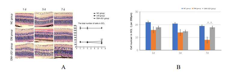
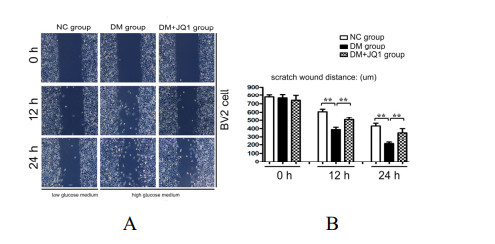
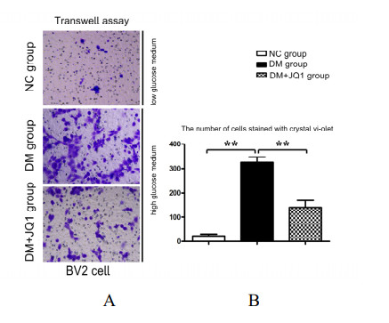
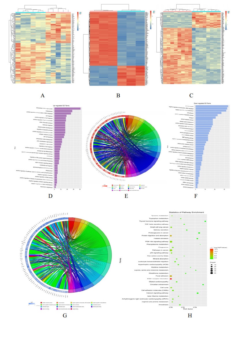
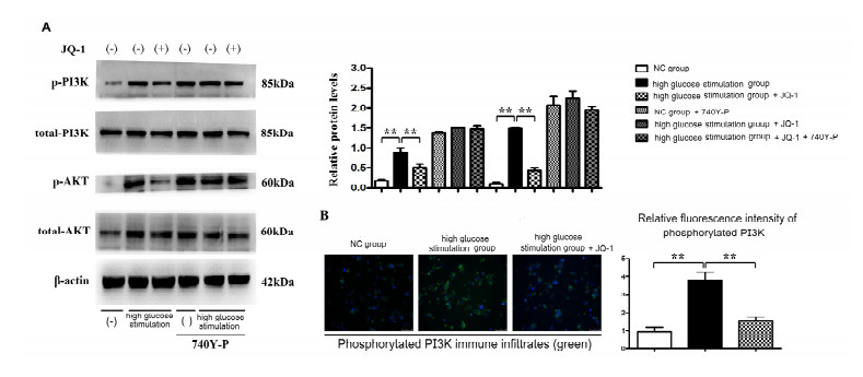
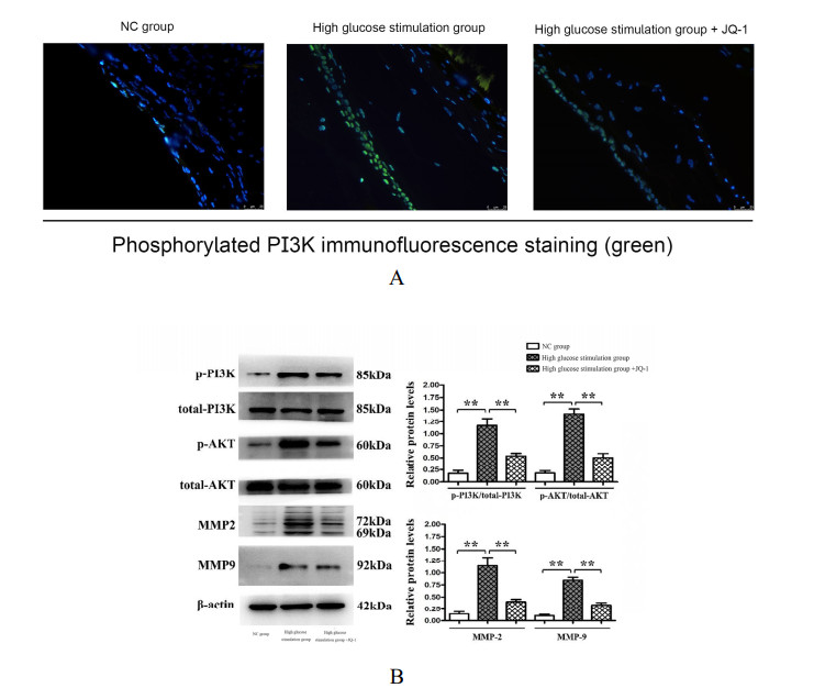
Diabetic retinopathy (DR) is one of the main leading causes of visual impairment worldwide. The current study elucidates the role of JQ1 in DR. A diabetic model was constructed by STZ injection and a high-fat diet. After establishment of the diabetic model, rats were assigned to treatment groups: 1) control, 2) diabetic model, and 3) diabetic+JQ1 model. In vitro Transwell and wound-healing assays were used to measure BV2 cell viability by stimulation with low glucose and high glucose with or without JQ1 and 740Y-P. Pathological methods were used to analyze DR, and Western blotting was used to analyze protein expression. Identification of enriched pathways in DR was performed by bioinformatics. Histopathological examination demonstrated that JQ1 rescued the loss of retinal cells and increased the thickness of retinal layers in diabetic rats. JQ1 attenuated high glucose-stimulated BV2 microglial motility and migration. The bioinformatics analysis implied that the Pl3K-Akt signaling pathway was enriched in DR. JQ1 decreased the phosphorylation of PI3K and AKT as well as the immunostaining of PI3K in BV2 cells. 740Y-P (a PI3K agonist) significantly reversed the decrease in p-PI3K and p-AK in BV2 cells. Additionally, JQ1 decreased the protein expression of p-PI3K, p-AKT, and MMP2/9 and immunostaining of PI3K in retinal tissues of rats. JQ1 suppresses the PI3K/Akt cascade by targeting MMP expression, thus decreasing the viability and invasion capacity of retinal microglia, suggesting an interesting treatment target for DR.
- JQ1,
- diabetic retinopathy,
- DR,
- PI3K/Akt,
- retinal microglia,
- RPs
Citation: Ying Zhu, Lipeng Guo, Jixin Zou, Liwen Wang, He Dong, Shengbo Yu, Lijun Zhang, Jun Li, Xueling Qu. JQ1 inhibits high glucose-induced migration of retinal microglial cells by regulating the PI3K/AKT signaling pathway[J]. Mathematical Biosciences and Engineering, 2022, 19(12): 13079-13092. doi: 10.3934/mbe.2022611

Related Papers:

Abstract

Diabetic retinopathy (DR) is one of the main leading causes of visual impairment worldwide. The current study elucidates the role of JQ1 in DR. A diabetic model was constructed by STZ injection and a high-fat diet. After establishment of the diabetic model, rats were assigned to treatment groups: 1) control, 2) diabetic model, and 3) diabetic+JQ1 model. In vitro Transwell and wound-healing assays were used to measure BV2 cell viability by stimulation with low glucose and high glucose with or without JQ1 and 740Y-P. Pathological methods were used to analyze DR, and Western blotting was used to analyze protein expression. Identification of enriched pathways in DR was performed by bioinformatics. Histopathological examination demonstrated that JQ1 rescued the loss of retinal cells and increased the thickness of retinal layers in diabetic rats. JQ1 attenuated high glucose-stimulated BV2 microglial motility and migration. The bioinformatics analysis implied that the Pl3K-Akt signaling pathway was enriched in DR. JQ1 decreased the phosphorylation of PI3K and AKT as well as the immunostaining of PI3K in BV2 cells. 740Y-P (a PI3K agonist) significantly reversed the decrease in p-PI3K and p-AK in BV2 cells. Additionally, JQ1 decreased the protein expression of p-PI3K, p-AKT, and MMP2/9 and immunostaining of PI3K in retinal tissues of rats. JQ1 suppresses the PI3K/Akt cascade by targeting MMP expression, thus decreasing the viability and invasion capacity of retinal microglia, suggesting an interesting treatment target for DR.

References

[1]	S. Babapoor-Farrokhran, K. Jee, B. Puchner, S. J. Hassan, X. Xin, M. Rodrigues, et al., Angiopoietin-like 4 is a potent angiogenic factor and a novel therapeutic target for patients with proliferative diabetic retinopathy, Proc. Natl. Acad. Sci., 112 (2015), 3030–3039. https://doi.org/10.1073/pnas.1423765112 doi: 10.1073/pnas.1423765112
[2]	Y. C. Chang, W. C. Wu, Dyslipidemia and diabetic retinopathy, Rev. Diabetic Stud., 10 (2012), 121–132. https://doi.org/10.1900/RDS.2013.10.121 doi: 10.1900/RDS.2013.10.121
[3]	L. Chen, C. Y. Cheng, H. Choi, M. K. Ikram, C. Sabanayagam, G. S. Tan, et al., Plasma metabonomic profiling of diabetic retinopathy, J. Am. Diabetes Assoc., 65 (2016), 1099–1108. https://doi.org/10.2337/db15-0661 doi: 10.2337/db15-0661
[4]	F. Semeraro, F. Morescalchi, A. Cancarini, A. Russo, S. Rezzola, C. Costagliola, Diabetic retinopathy, a vascular and inflammatory disease: Therapeutic implications, Diabetes Metab., 45 (2019), 517–527. https://doi.org/10.1016/j.diabet.2019.04.002 doi: 10.1016/j.diabet.2019.04.002
[5]	I. N. Mohamed, S. A. Soliman, A. Alhusban, S. Matragoon, B. A. Pillai, A. A. Elmarkaby, A. B. El-Remessy, Diabetes exacerbates retinal oxidative stress, inflammation, and microvascular degeneration in spontaneously hypertensive rats, Mol. Vision, 18 (2012), 1457–1466.
[6]	Z. Zhuang, H. Hu, S. Y. Tian, Z. J. Lu, T. Z. Zhang, Y. L. Bai, Down-regulation of microRNA-155 attenuates retinal neovascularization via the PI3K/Akt pathway, Mol. Vision, 21 (2015), 1173–1184.
[7]	B. Bahrami, M. Zhu, T. Hong, A. Chang, Diabetic macular oedema: pathophysiology, management challenges and treatment resistance, Diabetologia, 59 (2016), 1594–1608. https://doi.org/10.1007/s00125-016-3974-8 doi: 10.1007/s00125-016-3974-8
[8]	M. Henricsson, A. Nilsson, L. Janzon, L. Groop, The effect of glycaemic control and the introduction of insulin therapy on retinopathy in non-insulin-dependent diabetes mellitus, Diabetic Med., 14 (1997), 123–131. https://doi.org/10.1002/(SICI)1096-9136(199702)14:2<123::AID-DIA306>3.0.CO;2-U doi: 10.1002/(SICI)1096-9136(199702)14:2<123::AID-DIA306>3.0.CO;2-U
[9]	J. Yin, W. Q. Xu, M. X. Ye, Y. Zhang, H. Y. Wang, J. Zhang, et al., Up-regulated basigin-2 in microglia induced by hypoxia promotes retinal angiogenesis, J. Cell. Mol. Med., 7 (2017), 14925. https://doi.org/10.1111/jcmm.13256 doi: 10.1111/jcmm.13256
[10]	E. Kermorvant-Duchemin, A. C. Pinel, S. Lavalette, D. Lenne, W. Raoul, B. Calippe, et al., Neonatal hyperglycemia inhibits angiogenesis and induces inflammation and neuronal degeneration in the retina, PLoS ONE, 8 (2013), e79545. https://doi.org/10.1371/journal.pone.0079545 doi: 10.1371/journal.pone.0079545
[11]	X. Chen, H. Zhou, Y. Gong, S. Wei, M. Zhang, Early spatiotemporal characterization of microglial activation in the retinas of rats with streptozotocin-induced diabetes, Graefe's Arch. Clin. Exp. Ophthalmol., 253 (2015), 519–525. https://doi.org/10.1007/s00417-014-2727-y doi: 10.1007/s00417-014-2727-y
[12]	H. Qiu, A. L. Jackson, J. E. Kilgore, Y. Zhong, L. L. Y. Chan, P. A. Gehrig, et al., JQ1 suppresses tumor growth through downregulating LDHA in ovarian cancer, Oncotarget, 6 (2015), 6915. https://doi.org/10.18632/oncotarget.3126 doi: 10.18632/oncotarget.3126
[13]	H. Qiu, J. Li, L. H. Clark, A. L. Jackson, L. Zhang, H. Guo, et al., JQ1 suppresses tumor growth via PTEN/PI3K/AKT pathway in endometrial cancer, Oncotarget, 7 (2016), 66809–66821. https://doi.org/10.18632/oncotarget.11631 doi: 10.18632/oncotarget.11631
[14]	S. Bakshi, C. McKee, K. Walker, C. Brown, G. R. Chaudhry, Toxicity of JQ1 in neuronal derivatives of human umbilical cord mesenchymal stem cells, Oncotarget, 9 (2018), 33853–33864. https://doi.org/10.18632/oncotarget.26127 doi: 10.18632/oncotarget.26127
[15]	J. Mu, D. Zhang, Y. Tian, Z. Xie, M. H. Zou, et al., BRD4 inhibition by JQ1 prevents high-fat diet-induced diabetic cardiomyopathy by activating PINK1/Parkin-mediated mitophagy in vivo, J. Mol. Cell. Cardiol., 149 (2020). https://doi.org/10.1016/j.yjmcc.2020.09.003 doi: 10.1016/j.yjmcc.2020.09.003
[16]	Y. Wu, M. Zhang, C. Xu, D. Chai, F. Peng, J. Lin, Anti-diabetic atherosclerosis by inhibiting high glucose-induced vascular smooth muscle cell proliferation via Pin1/BRD4 pathway, Oxid. Med. Cell. Longevity, 2020 (2020), 1–13. https://doi.org/10.1155/2020/4196482 doi: 10.1155/2020/4196482
[17]	E. Liang, M. Ma, L. Wang, X. Liu, J. Xu, M. Zhang, The BET/BRD inhibitor JQ1 attenuates diabetes-induced cognitive impairment in rats by targeting Nox4-Nrf2 redox imbalance, Biochem. Biophys. Res. Commun., 2017, S0006291X17321976. https://doi.org/10.1016/j.bbrc.2017.11.020 doi: 10.1016/j.bbrc.2017.11.020
[18]	J. M. Zhou, S. S. Gu, W. H. Mei, J. Zhou, Z. Z. Wang, W. Xiao, Ginkgolides and bilobalide protect BV2 microglia cells against OGD/reoxygenation injury by inhibiting TLR2/4 signaling pathways, Cell Stress Chaperones, 21 (2016), 1037–1053. https://doi.org/10.1007/s12192-016-0728-y doi: 10.1007/s12192-016-0728-y
[19]	H. Shen, J. Zhang, Y. Zhang, Q. Feng, H. Wang, G. Li, et al., Knockdown of tripartite motif 59 (TRIM59) inhibits proliferation in cholangiocarcinoma via the PI3K/AKT/mTOR signalling pathway, Gene, 698 (2019), 50–60. https://doi.org/10.1016/j.gene.2019.02.044 doi: 10.1016/j.gene.2019.02.044
[20]	Z. Y. Sun, Y. K. Jian, H. Y. Zhu, B. Li, lncRNAPVT1 targets miR-152 to enhance chemoresistance of osteosarcoma to gemcitabine through activating c-MET/PI3K/AKT pathway, Pathol. Res. Pract., 215 (2019), 555–563. https://doi.org/10.1016/j.prp.2018.12.013 doi: 10.1016/j.prp.2018.12.013
[21]	D. S. Boyer, J. J. Hopkins, J. Sorof, J. S. Ehrlich, Anti-vascular endothelial growth factor therapy for diabetic macular edema, Ther. Adv. Endocrinol. Metab., 4 (2013), 151–169. https://doi.org/10.1177/2042018813512360 doi: 10.1177/2042018813512360
[22]	M. Ahmed, A. Asrar, Role of inflammation in the pathogenesis of diabetic retinopathy, Middle East Afr. J. Ophthalmol., 19 (2012), 70. https://doi.org/10.4103/0974-9233.92118 doi: 10.4103/0974-9233.92118
[23]	T. Bagratuni, N. Mavrianou, N. G. Gavalas, K. Tzannis, C. Arapinis, M. Liontos, et al., JQ1 inhibits tumour growth in combination with cisplatin and suppresses JAK/STAT signalling pathway in ovarian cancer, Eur. J. Cancer, 126 (2020), 125–135. https://doi.org/10.1016/j.ejca.2019.11.017 doi: 10.1016/j.ejca.2019.11.017
[24]	X. Xu, Y. Zong, Y. Gao, X. Sun, H. Zhao, W. Luo, et al., VEGF induce vasculogenic mimicry of choroidal melanoma through the PI3k signal pathway, BioMed Res. Int., 2019 (2019), 1–13. https://doi.org/10.1155/2019/3909102 doi: 10.1155/2019/3909102
[25]	N. Akeno, J. Robins, M. Zhang, M. F. Czyzyk-Krzeska, T. L. Clemens, Induction of vascular endothelial growth factor by IGF-I in osteoblast-like cells is mediated by the PI3K signaling pathway through the hypoxia-inducible factor-2alpha, Endocrinology, 143 (2002), 420–425. https://doi.org/10.1210/endo.143.2.8639 doi: 10.1210/endo.143.2.8639
[26]	M. Jafari, E. Ghadami, T. Dadkhah, H. Akhavan-Niaki, PI3k/AKT signaling pathway: Erythropoiesis and beyond, J. Cell. Physiol., 234 (2019), 2373–2385. https://doi.org/10.1002/jcp.27262 doi: 10.1002/jcp.27262

Reader Comments

Your name:*

Email:*
© 2022 the Author(s), licensee AIMS Press. This is an open access article distributed under the terms of the Creative Commons Attribution License (http://creativecommons.org/licenses/by/4.0)