Designing social distancing policies for the COVID-19 pandemic: A probabilistic model predictive control approach

Antonios Armaou; Bryce Katch; Lucia Russo; Constantinos Siettos; Antonios Armaou; Bryce Katch; Lucia Russo; Constantinos Siettos

doi:10.3934/mbe.2022409

Mathematical Biosciences and Engineering

2022, Volume 19, Issue 9: 8804-8832. doi: 10.3934/mbe.2022409

Previous Article Next Article

Research article Special Issues

Designing social distancing policies for the COVID-19 pandemic: A probabilistic model predictive control approach

1.
Dept. of Chemical Engineering, The Pennsylvania State University, USA
2.
Institute of Science and Technology for Energy and Sustainable Mobility, Consiglio Nazionale delle Ricerche, Italy
3.
Dipartimento di Matematica e Applicazioni "Renato Caccioppoli", Scuola Superiore Meridionale, Università degli Studi di Napoli Federico Ⅱ, Naples, Italy

Received: 15 December 2021 Revised: 25 January 2022 Accepted: 07 February 2022 Published: 17 June 2022

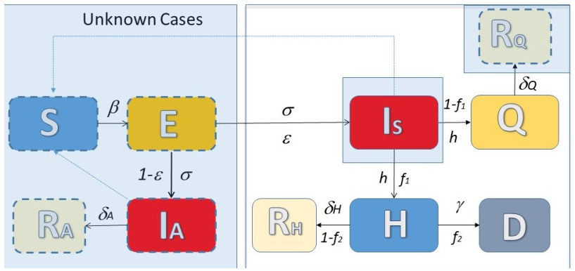
The effective control of the COVID-19 pandemic is one the most challenging issues of recent years. The design of optimal control policies is challenging due to a variety of social, political, economical and epidemiological factors. Here, based on epidemiological data reported in recent studies for the Italian region of Lombardy, which experienced one of the largest and most devastating outbreaks in Europe during the first wave of the pandemic, we present a probabilistic model predictive control (PMPC) approach for the systematic study of what if scenarios of social distancing in a retrospective analysis for the first wave of the pandemic in Lombardy. The performance of the proposed PMPC was assessed based on simulations of a compartmental model that was developed to quantify the uncertainty in the level of the asymptomatic cases in the population, and the synergistic effect of social distancing during various activities, and public awareness campaign prompting people to adopt cautious behaviors to reduce the risk of disease transmission. The PMPC takes into account the social mixing effect, i.e. the effect of the various activities in the potential transmission of the disease. The proposed approach demonstrates the utility of a PMPC approach in addressing COVID-19 transmission and implementing public relaxation policies.
- COVID-19 pandemic,
- model predictive control,
- forecasting,
- Lombardy Italy,
- social distancing,
- social mixing,
- Google mobility reports
Citation: Antonios Armaou, Bryce Katch, Lucia Russo, Constantinos Siettos. Designing social distancing policies for the COVID-19 pandemic: A probabilistic model predictive control approach[J]. Mathematical Biosciences and Engineering, 2022, 19(9): 8804-8832. doi: 10.3934/mbe.2022409

Related Papers:

Abstract

The effective control of the COVID-19 pandemic is one the most challenging issues of recent years. The design of optimal control policies is challenging due to a variety of social, political, economical and epidemiological factors. Here, based on epidemiological data reported in recent studies for the Italian region of Lombardy, which experienced one of the largest and most devastating outbreaks in Europe during the first wave of the pandemic, we present a probabilistic model predictive control (PMPC) approach for the systematic study of what if scenarios of social distancing in a retrospective analysis for the first wave of the pandemic in Lombardy. The performance of the proposed PMPC was assessed based on simulations of a compartmental model that was developed to quantify the uncertainty in the level of the asymptomatic cases in the population, and the synergistic effect of social distancing during various activities, and public awareness campaign prompting people to adopt cautious behaviors to reduce the risk of disease transmission. The PMPC takes into account the social mixing effect, i.e. the effect of the various activities in the potential transmission of the disease. The proposed approach demonstrates the utility of a PMPC approach in addressing COVID-19 transmission and implementing public relaxation policies.

References

[1]	Johns Hopkins Center for Health Security, Coronavirus COVID-19 Global Cases by Johns Hopkins CSSE, Feb 2020.
[2]	C. Anastassopoulou, C. Siettos, L. Russo, G. Vrioni, A. Tsakris, Lessons from the devastating impact of the first COVID-19 wave in Italy, Pathog. Glob. Health, 12 (2021), 211–212. https://doi.org/10.1080/20477724.2021.1894399 doi: 10.1080/20477724.2021.1894399
[3]	Google. Community Mobility Reports, 2020.
[4]	M. V. Corazza, L. Moretti, G. Forestieri, G. Galiano, Chronicles from the new normal: Urban planning, mobility and land-use management in the face of the COVID-19 crisis, Transp. Res. Inter. Persp., 12 (2021), 10050. https://doi.org/10.1016/j.trip.2021.100503 doi: 10.1016/j.trip.2021.100503
[5]	S. Zhao, Q. Lin, J. Ran, S. S. Musa, G. Yang, W. Wang, et al., Preliminary estimation of the basic reproduction number of novel coronavirus (2019-nCoV) in china, from 2019 to 2020: A data-driven analysis in the early phase of the outbreak, Int. J. Inf. Dis, 92 (2020), 214–217. https://doi.org/10.1016/j.ijid.2020.01.050 doi: 10.1016/j.ijid.2020.01.050
[6]	A. Remuzzi, G. Remuzzi, COVID-19 and Italy: What next? The Lancet, 395 (2020), 1225–1228. https://doi.org/10.1016/S0140-6736(20)30627-9 doi: 10.1016/S0140-6736(20)30627-9
[7]	J. T. Wu, K. Leung, G. M. Leung, Nowcasting and forecasting the potential domestic and international spread of the 2019-nCoV outbreak originating in Wuhan, China: A modelling study, The Lancet, 395 (2020), 689–697. https://doi.org/10.1016/S0140-6736(20)30260-9 doi: 10.1016/S0140-6736(20)30260-9
[8]	C. Anastassopoulou, L. Russo, A. Tsakris, C. Siettos, Data-based analysis, modelling and forecasting of the COVID-19 outbreak, PLoS ONE, 15 (2020), e0230405. https://doi.org/10.1371/journal.pone.0230405 doi: 10.1371/journal.pone.0230405
[9]	Y. Belgaid, M. Helal, E. Venturino, Analysis of a model for coronavirus spread, Mathematics, 8 (2020), 820. https://doi.org/10.3390/math8050820 doi: 10.3390/math8050820
[10]	L. Russo, C. Anastassopoulou, A. Tsakris, G.N. Bifulco, E.F. Campana, G. Toraldo, et al., Tracing day-zero and forecasting the COVID-19 outbreak in lombardy, Italy: A compartmental modelling and numerical optimization approach, PloS One, 15 (2020), e0240649. https://doi.org/10.1371/journal.pone.0240649 doi: 10.1371/journal.pone.0240649
[11]	M. Chinazzi, J. T. Davis, M. Ajelli, G. Gioannini, M. Litvinova, S. Merler, et al., The effect of travel restrictions on the spread of the 2019 novel coronavirus (COVID-19) outbreak, Science, 368 (2020), 395–400. https://doi.org/10.1126/science.aba9757 doi: 10.1126/science.aba9757
[12]	F. Di Lauro, I. Z. Kiss, D. Rus, C. Della Santina, COVID-19 and flattening the curve: A feedback control perspective, IEEE Control Sys. Lett., 5 (2021), 1435–1440. https://doi.org/10.1109/LCSYS.2020.3039322 doi: 10.1109/LCSYS.2020.3039322
[13]	J. Köhler, L. Schwenkel, A. Koch, J. Berberich, P. Pauli, F. Allgöwer, Robust and optimal predictive control of the COVID-19 outbreak, Ann. Rev. Control, 51 (2021), 525–539. https://doi.org/10.1016/j.arcontrol.2020.11.002 doi: 10.1016/j.arcontrol.2020.11.002
[14]	M. A. Hadi, H. Ali I, Control of COVID-19 system using a novel nonlinear robust control algorithm, Biom. Signal Proc. Control, 64 (2021), 102317. https://doi.org/10.1016/j.bspc.2020.102317 doi: 10.1016/j.bspc.2020.102317
[15]	T. Peni, B. Csutak, G. Szederkenyi, G. Rost, Nonlinear model predictive control with logic constraints for COVID-19 management, Non. Dyn., 102 (2020), 1965–1986. https://doi.org/10.1007/s11071-020-05980-1 doi: 10.1007/s11071-020-05980-1
[16]	R. Carli, G. Cavone, N. Epicoco, P. Scarabaggio, M. Dotoli, Model predictive control to mitigate the COVID-19 outbreak in a multi-region scenario, Annual Rev. Control, 50 (2020), 373–393. https://doi.org/10.1016/j.arcontrol.2020.09.005 doi: 10.1016/j.arcontrol.2020.09.005
[17]	C. Tsay, F. Lejarza, M. A. Stadtherr, M. Baldea, Modeling, state estimation, and optimal control for the US COVID-19 outbreak, Sci. Rep., 10 (2020), 10711. https://doi.org/10.1038/s41598-020-67459-8 doi: 10.1038/s41598-020-67459-8
[18]	F. Della Rossa, D. Salzano, A. Di Meglio, F. De Lellis, M. Coraggio, C. Calabrese, et al., A network model of Italy shows that intermittent regional strategies can alleviate the COVID-19 epidemic, Nat. Comm., 11 (2020), 1–9. https://doi.org/10.1038/s41467-019-13993-7 doi: 10.1038/s41467-019-13993-7
[19]	J. Mossong, N. Hens, M. Jit, P. Beutels, K. Auranen, R. Mikolajczyk, et al., Social contacts and mixing patterns relevant to the spread of infectious diseases, PLoS Med., 5 (2008), e74. https://doi.org/10.1371/journal.pmed.0050074 doi: 10.1371/journal.pmed.0050074
[20]	F. M. Grosso, A. M. Presanis, K. Kunzmann, C. Jackson, A. Corbella, G. Grasselli, et al., Decreasing hospital burden of COVID-19 during the first wave in regione Lombardia: An emergency measures context, Morb. Mortality Weekly Rep., 3 (2021), 1612. https://doi.org/10.21203/rs.3.rs-288193/v1 doi: 10.21203/rs.3.rs-288193/v1
[21]	V. Marziano, G. Guzzetta, B. M. Rondinone, F. Boccuni, F. Riccardo, A. Bella, et al., Retrospective analysis of the italian exit strategy from COVID-19 lockdown, PNAS, 118 (2021), e2019617118. https://doi.org/10.1073/pnas.2019617118 doi: 10.1073/pnas.2019617118
[22]	A. Fochesato, G. Simoni, F. Reali, G. Giordano, E. Domenici, L. Marchetti, A retrospective analysis of the COVID-19 pandemic evolution in Italy, Biology, 10 (2021), 311. https://doi.org/10.3390/biology10040311 doi: 10.3390/biology10040311
[23]	J. Osborn, S. Berman, S. Bender-Bier, G. D'Souza, M. Myers, Retrospective analysis of interventions to epidemics using dynamic simulation of population behavior, Math. Biosci., 341 (2021), 108712. https://doi.org/10.1016/j.mbs.2021.108712 doi: 10.1016/j.mbs.2021.108712
[24]	Il messaggero. Coronavirus, stop ai test facili: Tampone solo a chi ha i sintomi, 2020.
[25]	E. Chung, E. Chow, N. Wilcox, R. Burstein, E. Brandstetter, P.D. Han, et al., Comparison of symptoms and RNA levels in children and adults with SARS-CoV-2 infection in the community setting, JAMA Pediatr., 175 (2021), e212025. https://doi.org/10.1001/jamapediatrics.2021.2025 doi: 10.1001/jamapediatrics.2021.2025
[26]	Q. Li, X. Guan, P. Wu, X. Wang, L. Zhou, Y. Tong, et al., Early transmission dynamics in Wuhan, China, of novel coronavirus infected pneumonia, New Engl. J. Med., 382 (2020), 1199–1207. https://doi.org/10.1056/NEJMoa2001316 doi: 10.1056/NEJMoa2001316
[27]	X. He, E. H. Lau, P. Wu, X. Deng, J. Wang, X. Hao, et al., Temporal dynamics in viral shedding and transmissibility of COVID-19, Nat. Med., 26 (2020), 672–675. https://doi.org/10.1038/s41591-020-0869-5 doi: 10.1038/s41591-020-0869-5
[28]	I. Istituto Superiore di Sanit, Characteristics of SARS-CoV-2 patients dying in Italy Report based on available data on December 16th, 2020, 2020.
[29]	D. Cereda, M. Manica, M. Tirani, F. Rovida, V. Demicheli, M. Ajelli, et al., The early phase of the COVID-19 epidemic in Lombardy, Italy, Epidemics, 37 (2021), 100528. https://doi.org/10.1016/j.epidem.2021.100528 doi: 10.1016/j.epidem.2021.100528
[30]	Q. Bi, Y. Wu, S. Mei, C. Ye, X. Zou, Z. Zhang, et al., Epidemiology and transmission of COVID-19 in 391 cases and 1286 of their close contacts in Shenzhen, China: A retrospective cohort study, The Lancet Infect. Dis., 20 (2020), 911–919. https://doi.org/10.1016/S1473-3099(20)30287-5 doi: 10.1016/S1473-3099(20)30287-5
[31]	J. Chen, T. Qi, L. Liu, Y. Ling, Z. Qian, T. Li, et al., Clinical progression of patients with COVID-19 in Shanghai, China, J. Infect., 80 (2020), e1–e6. https://doi.org/10.1016/j.jinf.2020.03.004 doi: 10.1016/j.jinf.2020.03.004
[32]	Italy Istituto Superiore di Sanit. Characteristics of COVID-19 patients dying in Italy Report based on available data on March 20th, 2020, 2020.
[33]	G. Sartor, M. Del Riccio, I. Dal Poz, P. Bonanni, G. Bonaccorsi, COVID-19 in Italy: Considerations on official data, Int. J. Inf. Dis., 98 (2020), 188–190. https://doi.org/10.1016/j.ijid.2020.06.060 doi: 10.1016/j.ijid.2020.06.060
[34]	E. Ferroni, P. G. Rossi, S. S. Alegiani, G. Trifirò, G. Pitter, O. Leoni, et al., Survival of hospitalized COVID-19 patients in northern italy: A population-based cohort study by the ITA-COVID-19 network, Clin. Epidemiol., 12 (2020), 1337. https://doi.org/10.2147/CLEP.S271763 doi: 10.2147/CLEP.S271763
[35]	G. Zehender, A. Lai, A. Bergna, L. Meroni, A. Riva, C. Balotta, et al., Genomic characterisation and phylogenetic analysis of sars-cov-2 in Italy, J. Med. Vir., 92 (2020), 1637–1640. https://doi.org/10.1002/jmv.25794 doi: 10.1002/jmv.25794
[36]	E. I. Jury, L. Stark, V. V. Krishnan, Inners and stability of dynamic systems, IEEE Trans. Sys. Man Cyb., SMC-6 (1976), 724–725. https://doi.org/10.1109/TSMC.1976.4309436 doi: 10.1109/TSMC.1976.4309436
[37]	M. Allieta, A. Allieta, D. R. Sebastiano, COVID-19 outbreak in Italy: estimation of reproduction numbers over 2 months prior to phase 2, J. Public Health, 1–9.
[38]	M. D'Arienzo, A. Coniglio, Assessment of the SARS-COV-2 basic reproduction number, R0, based on the early phase of COVID-19 outbreak in Italy, Biosaf. Health, 2 (2020), 57–59. https://doi.org/10.1016/j.bsheal.2020.03.004 doi: 10.1016/j.bsheal.2020.03.004
[39]	G. Pillonetto, M. Bisiacco, G. Palù, C. Cobelli, Tracking the time course of reproduction number and lockdown's effect on human behaviour during SARS-COV-2 epidemic: Nonparametric estimation, Sci. Rep., 11 (2021), 1–16. https://doi.org/10.1038/s41598-021-89014-9 doi: 10.1038/s41598-021-89014-9
[40]	A. Cori, N. M. Ferguson, C. Fraser, S. Cauchemez, A new framework and software to estimate time-varying reproduction numbers during epidemics, Am. J. Epidemiol., 178 (2013), 1505–1512. https://doi.org/10.1093/aje/kwt133 doi: 10.1093/aje/kwt133
[41]	D. A. Armstrong, M. J. Lebo, J. Lucas, Do COVID-19 policies affect mobility behaviour? evidence from 75 canadian and american cities, Can. Public Policy, 46 (2020), S127–S144. https://doi.org/10.3138/cpp.2020-062 doi: 10.3138/cpp.2020-062
[42]	B. Buonomo, R. Della Marca, Effects of information-induced behavioural changes during the COVID-19 lockdowns: The case of Italy, Royal Soc. Open Sci., 7 (2020), 201635. https://doi.org/10.1098/rsos.201635 doi: 10.1098/rsos.201635
[43]	H. S. Badr, H. Du, M. Marshall, E. Dong, M. M. Squire, L. M. Gardner, Association between mobility patterns and COVID-19 transmission in the USA: A mathematical modelling study, Lancet Inf. Dis., 20 (2020), 1247–1254. https://doi.org/10.1016/S1473-3099(20)30553-3 doi: 10.1016/S1473-3099(20)30553-3
[44]	M. Vollmer, S. Mishra, J. Unwin, A. Gandy, T.A. Mellan, V. Bradley, et al., Report 20: Using mobility to estimate the transmission intensity of COVID-19 in Italy: A subnational analysis with future scenarios, medRxiv.
[45]	P. Caley, D. J. Philp, K. McCracken, Quantifying social distancing arising from pandemic influenza, J. Royal Soc. Int., 5 (2007), 631–639. https://doi.org/10.1098/rsif.2007.1197 doi: 10.1098/rsif.2007.1197
[46]	P. Mhaskar, N. H. El-Farra, P. D. Christofides, Robust hybrid predictive control of nonlinear systems, Automatica, 41 (2005), 209–217. https://doi.org/10.1016/j.automatica.2004.08.020 doi: 10.1016/j.automatica.2004.08.020
[47]	V. Volpert, M. Banerjee, A. d'Onofrio, T. Lipniacki, S. Petrovskii, V. C. Tran, Coronavirus - scientific insights and societal aspects, Math. Model. Nat. Phenom., 15 (2020), 188–190. https://doi.org/10.1051/mmnp/2020010 doi: 10.1051/mmnp/2020010
[48]	K. B. Blyuss, Y. N. Kyrychko, Effects of latency and age structure on the dynamics and containment of COVID-19, J. Theor. Biol., 513 (2021), 110587. https://doi.org/10.1016/j.jtbi.2021.110587 doi: 10.1016/j.jtbi.2021.110587
[49]	Alberto d'Onofrio (ed.), Bounded Noises in Physics, Biology, and Engineering, Springer New York, 2013.
[50]	P. Mhaskar, N. El-Farra, P. Christofides, Predictive control of switched nonlinear systems with scheduled mode transitions, IEEE Trans. Aut. Control, 50 (2005), 1670–1680. https://doi.org/10.1109/TAC.2005.858692 doi: 10.1109/TAC.2005.858692

Reader Comments

Your name:*

Email:*
© 2022 the Author(s), licensee AIMS Press. This is an open access article distributed under the terms of the Creative Commons Attribution License (http://creativecommons.org/licenses/by/4.0)