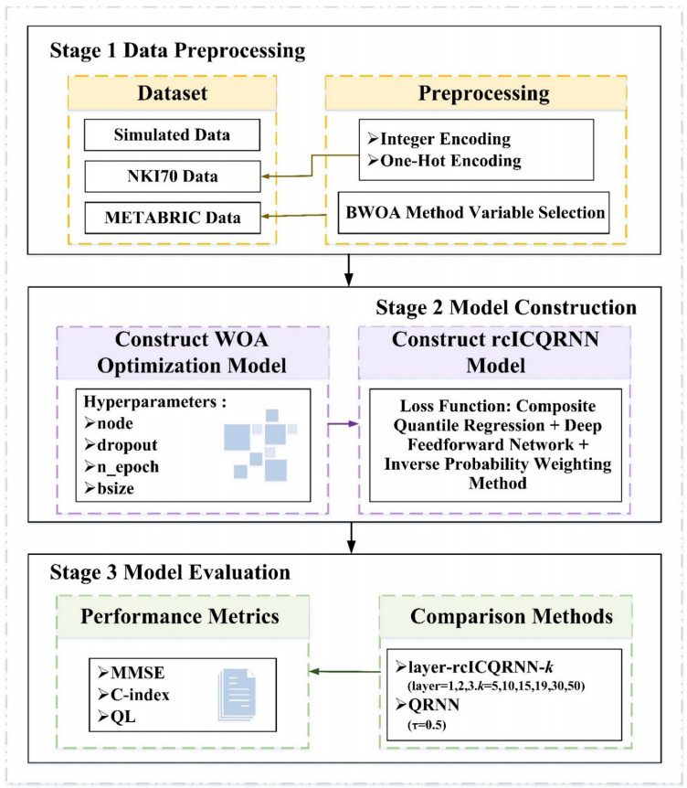
With the development of the field of survival analysis, statistical inference of right-censored data is of great importance for the study of medical diagnosis. In this study, a right-censored data survival prediction model based on an improved composite quantile regression neural network framework, called rcICQRNN, is proposed. It incorporates composite quantile regression with the loss function of a multi-hidden layer feedforward neural network, combined with an inverse probability weighting method for survival prediction. Meanwhile, the hyperparameters involved in the neural network are adjusted using the WOA algorithm, integer encoding and One-Hot encoding are implemented to encode the classification features, and the BWOA variable selection method for high-dimensional data is proposed. The rcICQRNN algorithm was tested on a simulated dataset and two real breast cancer datasets, and the performance of the model was evaluated by three evaluation metrics. The results show that the rcICQRNN-5 model is more suitable for analyzing simulated datasets. The One-Hot encoding of the WOA-rcICQRNN-30 model is more applicable to the NKI70 data. The model results are optimal for $ k = 15 $ after feature selection for the METABRIC dataset. Finally, we implemented the method for cross-dataset validation. On the whole, the Cindex results using One-Hot encoding data are more stable, making the proposed rcICQRNN prediction model flexible enough to assist in medical decision making. It has practical applications in areas such as biomedicine, insurance actuarial and financial economics.
Citation: Xiwen Qin, Dongmei Yin, Xiaogang Dong, Dongxue Chen, Shuang Zhang. Survival prediction model for right-censored data based on improved composite quantile regression neural network[J]. Mathematical Biosciences and Engineering, 2022, 19(8): 7521-7542. doi: 10.3934/mbe.2022354
With the development of the field of survival analysis, statistical inference of right-censored data is of great importance for the study of medical diagnosis. In this study, a right-censored data survival prediction model based on an improved composite quantile regression neural network framework, called rcICQRNN, is proposed. It incorporates composite quantile regression with the loss function of a multi-hidden layer feedforward neural network, combined with an inverse probability weighting method for survival prediction. Meanwhile, the hyperparameters involved in the neural network are adjusted using the WOA algorithm, integer encoding and One-Hot encoding are implemented to encode the classification features, and the BWOA variable selection method for high-dimensional data is proposed. The rcICQRNN algorithm was tested on a simulated dataset and two real breast cancer datasets, and the performance of the model was evaluated by three evaluation metrics. The results show that the rcICQRNN-5 model is more suitable for analyzing simulated datasets. The One-Hot encoding of the WOA-rcICQRNN-30 model is more applicable to the NKI70 data. The model results are optimal for $ k = 15 $ after feature selection for the METABRIC dataset. Finally, we implemented the method for cross-dataset validation. On the whole, the Cindex results using One-Hot encoding data are more stable, making the proposed rcICQRNN prediction model flexible enough to assist in medical decision making. It has practical applications in areas such as biomedicine, insurance actuarial and financial economics.

| [1] |
P. Wang, Y. Li, C. K. Reddy, Machine learning for survival analysis, ACM Comput. Surv., 51 (2019), 1-36. https://doi.org/10.1145/3214306 doi: 10.1145/3214306

|
| [2] |
E. L. Kaplan, P. Meier, Nonparametric estimation from incomplete observations, J. Am. Stat. Assoc., 53 (1958), 457-481. https://doi.org/10.2307/2281868 doi: 10.2307/2281868
|
| [3] |
J. H. Shows, W. Lu, H. Z. Hao, Sparse estimation and inference for censored median regression, J. Stat. Plann. Inference, 140 (2010), 1903-1917. https://doi.org/10.1016/j.jspi.2010.01.043 doi: 10.1016/j.jspi.2010.01.043
|
| [4] |
A. Giussani, M. Bonetti, Marshall—Olkin frailty survival models for bivariate right-censored failure time data, J. Appl. Stat., 46 (2019), 2945-2961. https://doi.org/10.1080/02664763.2019.1624694 doi: 10.1080/02664763.2019.1624694
|
| [5] |
Q. Yu, The MLE of the uniform distribution with right-censored data, Lifetime Data Anal., 27 (2021), 1-17. https://doi.org/10.1007/s10985-021-09528-2 doi: 10.1007/s10985-021-09528-2
|
| [6] |
R. Koenker, G. W. Bassett, Regression quantiles, Econometrica, 46 (1978), 33-50. https://doi.org/10.2307/1913643 doi: 10.2307/1913643
|
| [7] |
H. Zou, M. Yuan, Composite quantile regression and the oracle model selection theory, Ann. Stat., 36 (2008), 1108-1126. https://doi.org/10.1214/07-AOS507 doi: 10.1214/07-AOS507
|
| [8] |
J. Shim, C. Hwang, K. Seok, Composite support vector quantile regression estimation, Comput. Stat., 29 (2014), 1651-1665. https://doi.org/10.1007/s00180-014-0511-4 doi: 10.1007/s00180-014-0511-4
|
| [9] |
S. Bang, H. Cho, M. Jhun, Adaptive lasso penalised censored composite quantile regression, Int. J. Data Min. Bioinf., 15 (2016), 22-46. https://doi.org/10.1504/IJDMB.2016.076015 doi: 10.1504/IJDMB.2016.076015
|
| [10] |
S. Bang, S. H. Eo, M. Jhun, H. J. Cho, Composite kernel quantile regression, Commun. Stat. Simul. Comput., 46 (2016), 2228-2240. https://doi.org/10.1080/03610918.2015.1039133 doi: 10.1080/03610918.2015.1039133
|
| [11] |
Q. Xu, K. Deng, C. Jiang, F. Sun, X. Huang, Composite quantile regression neural network with applications, Expert Syst. Appl., 76 (2017), 129-139. https://doi.org/10.1016/j.eswa.2017.01.054 doi: 10.1016/j.eswa.2017.01.054
|
| [12] |
J. Wang, W. Jiang, F. Xu, W. Fu, Weighted composite quantile regression with censoring indicators missing at random, Commun. Stat. Theory Methods, 50 (2019), 1-18. https://doi.org/10.1080/03610926.2019.1678638 doi: 10.1080/03610926.2019.1678638
|
| [13] |
L. M. De, P. M. Ravdin, Survival analysis of censored data: Neural network analysis detection of complex interactions between variables, Breast Cancer Res. Treat., 32 (1994), 113-118. https://doi.org/10.1007/BF00666212 doi: 10.1007/BF00666212
|
| [14] |
J. L. Katzman, U. Shaham, A. Cloninger, J. Bates, Y. Kluger, DeepSurv: Personalized treatment recommender system using a Cox proportional hazards deep neural network, BMC Med. Res. Method., 18(2018), 24. https://doi.org/10.1186/s12874-018-0482-1 doi: 10.1186/s12874-018-0482-1
|
| [15] |
C. Anika, G. Olivier, Deep learning with multimodal representation for pancancer prongosis prediction, Bioinformatics, 35 (2019), i446-i454. https://doi.org/10.1093/bioinformatics/btz342 doi: 10.1093/bioinformatics/btz342
|
| [16] |
J. Wang, N. Chen, J. Guo, X. Xu, Z. Yi, SurvNet: A novel deep neural network for lung cancer survival analysis with missing values, Front. Oncol., 10 (2021), 588990-588990. https://doi.org/10.3389/FONC.2020.588990 doi: 10.3389/FONC.2020.588990
|
| [17] |
J. H. Oh, W. Choi, E. Ko, M. Kang, A. Tannenbaum, J. O. Deasy, PathCNN: Interpretable convolutional neural networks for survival prediction and pathway analysis applied to glioblastoma, Bioinformatics, 37 (2021), i443-i450. https://doi.org/10.1093/BIOINFORMATICS/BTAB285 doi: 10.1093/BIOINFORMATICS/BTAB285
|
| [18] |
B. Ma, G. Yan, B. Chai, X. Hou, XGBLC: An improved survival prediction model based on XGBoost, Bioinformatics, 38 (2021), 410-418. https://doi.org/10.1093/bioinformatics/btab675. doi: 10.1093/bioinformatics/btab675
|
| [19] |
N. Arya, S. Saha, Multi-modal advanced deep learning architectures for breast cancer survival prediction, Knowl. Based Syst., 221 (2021), 106965. https://doi.org/10.1016/J.KNOSYS.2021.106965 doi: 10.1016/J.KNOSYS.2021.106965
|
| [20] |
S. M. Zahra, M. Alexa, A two-stage modeling approach for breast cancer survivability prediction, Int. J. Med. Inf., 149 (2021), 104438. https://doi.org/10.1016/J.IJMEDINF.2021.104438 doi: 10.1016/J.IJMEDINF.2021.104438
|
| [21] |
Y. Jia, J. H. Jeong, Deep learning for quantile regression under right censoring: DeepQuantreg, Comput. Stat. Data Anal., 165 (2022), 107323. https://doi.org/10.1016/J.CSDA.2021.107323 doi: 10.1016/J.CSDA.2021.107323
|
| [22] |
J. W. Taylor, A quantile regression neural network approach to estimating the conditional density of multiperiod returns, J. Forecasting, 19 (2000), 299-311. https://doi.org/10.1002/1099-131X(200007)19:4<299::AID-FOR775>3.0.CO;2-V doi: 10.1002/1099-131X(200007)19:4<299::AID-FOR775>3.0.CO;2-V
|
| [23] |
A. J. Cannon, Quantile regression neural networks: Implementation in r and application to precipitation downscaling, Comput. Geosci., 37 (2011), 1277-1284. https://doi.org/10.1016/j.cageo.2010.07.005 doi: 10.1016/j.cageo.2010.07.005
|
| [24] |
P. J. Huber, Robust Regression: Asymptotics, Conjectures and Monte Carlo, Ann. Stat., 1 (1973), 799-821. https://doi.org/10.1214/aos/1176342503 doi: 10.1214/aos/1176342503
|
| [25] | H. Jian, S. Ma, H. Xie, Least absolute deviations estimation for the accelerated failure time model, Stat. Sin., 17 (2007), 1533-1548. https://www.jstor.org/stable/24307687 |
| [26] |
S. Mirjalili, A. Lewis, The whale optimization algorithm, Adv. Eng. Software, 95 (2016), 51-67. https://doi.org/10.1016/j.advengsoft.2016.01.008 doi: 10.1016/j.advengsoft.2016.01.008
|
| [27] |
W. Zheng, X. Peng, D. Lu, D. Zhang, Y. Liu, Z. Lin, et al, Composite quantile regression extreme learning machine with feature selection for short-term wind speed forecasting: A new approach, Energy Convers. Manage., 151 (2017), 737-752. https://doi.org/10.1016/j.enconman.2017.09.029 doi: 10.1016/j.enconman.2017.09.029
|
| [28] | F. E. Harrell, K. L. Lee, D. B. Mark, Multivariable prognostic models: Issues in developing models, evaluating assumptions and adequacy, and measuring and reducing errors, Stat. Med., 15 (1996), 361-687. https://doi.org/10.1002/(SICI)1097-0258(19960229)15:4<361::AID-SIM168>3.0.CO;2-4 |
| [29] |
P. C. Austin, Generating survival times to simulate Cox proportional hazards models with time-varying covariates, Stat. Med., 31(2012), 3946-3958. https://doi.org/10.1002/sim.5452 doi: 10.1002/sim.5452
|
| [30] |
T. Hanaa, A. Mostafa, E. Nawal, S. Hanaa, A novel deep autoencoder based survival analysis approach for microarray dataset, PeerJ Comput. Sci., 7 (2021), e492-e492. https://doi.org/10.7717/PEERJ-CS.492 doi: 10.7717/PEERJ-CS.492
|
| [31] |
E. Biganzoli, P. Boracchi, L. Mariani, E. Marubini, Feed forward neural networks for the analysis of censored survival data: A partial logistic regression approach, Stat. Med., 17 (1998), 1169-1186. https://doi.org/10.1002/(SICI)1097-0258(19980530)17:10<1169::AID-SIM796>3.0.CO;2-D doi: 10.1002/(SICI)1097-0258(19980530)17:10<1169::AID-SIM796>3.0.CO;2-D
|
| [32] |
P. J. G. Lisboa, H. Wong, P. Harris, R. Swindell, A Bayesian neural network approach for modelling censored data with an application to prognosis after surgery for breast cancer, Artif. Intell. Med., 28 (2003), 1-25. https://doi.org/10.1016/S0933-3657(03)00033-2 doi: 10.1016/S0933-3657(03)00033-2
|
 mbe-19-08-354-supplementary.pdf mbe-19-08-354-supplementary.pdf |
 |
Figures(5) / Tables(6)

Xiwen Qin, Dongmei Yin, Xiaogang Dong, Dongxue Chen, Shuang Zhang. Survival prediction model for right-censored data based on improved composite quantile regression neural network[J]. Mathematical Biosciences and Engineering, 2022, 19(8): 7521-7542. doi: 10.3934/mbe.2022354


 DownLoad: