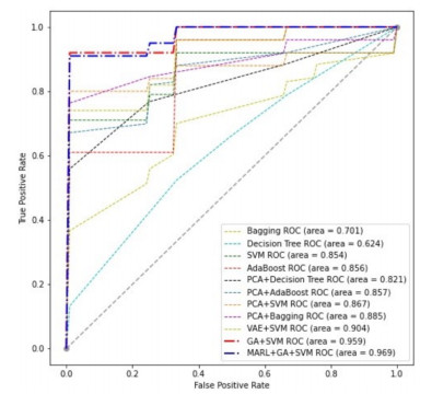
The neuropsychiatric systemic lupus erythematosus (NPSLE), a severe disease that can damage the heart, liver, kidney, and other vital organs, often involves the central nervous system and even leads to death. Magnetic resonance spectroscopy (MRS) is a brain functional imaging technology that can detect the concentration of metabolites in organs and tissues non-invasively. However, the performance of early diagnosis of NPSLE through conventional MRS analysis is still unsatisfactory. In this paper, we propose a novel method based on genetic algorithm (GA) and multi-agent reinforcement learning (MARL) to improve the performance of the NPSLE diagnosis model. Firstly, the proton magnetic resonance spectroscopy ($ ^{1} $H-MRS) data from 23 NPSLE patients and 16 age-matched healthy controls (HC) were standardized before training. Secondly, we adopt MARL by assigning an agent to each feature to select the optimal feature subset. Thirdly, the parameter of SVM is optimized by GA. Our experiment shows that the SVM classifier optimized by feature selection and parameter optimization achieves 94.9% accuracy, 91.3% sensitivity, 100% specificity and 0.87 cross-validation score, which is the best score compared with other state-of-the-art machine learning algorithms. Furthermore, our method is even better than other dimension reduction ones, such as SVM based on principal component analysis (PCA) and variational autoencoder (VAE). By analyzing the metabolites obtained by MRS, we believe that this method can provide a reliable classification result for doctors and can be effectively used for the early diagnosis of this disease.
Citation: Guanru Tan, Boyu Huang, Zhihan Cui, Haowen Dou, Shiqiang Zheng, Teng Zhou. A noise-immune reinforcement learning method for early diagnosis of neuropsychiatric systemic lupus erythematosus[J]. Mathematical Biosciences and Engineering, 2022, 19(3): 2219-2239. doi: 10.3934/mbe.2022104
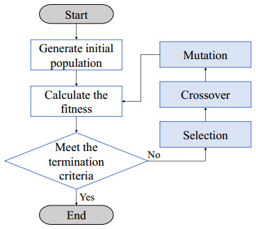
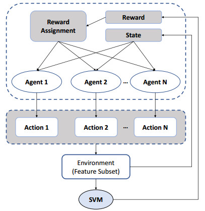
The neuropsychiatric systemic lupus erythematosus (NPSLE), a severe disease that can damage the heart, liver, kidney, and other vital organs, often involves the central nervous system and even leads to death. Magnetic resonance spectroscopy (MRS) is a brain functional imaging technology that can detect the concentration of metabolites in organs and tissues non-invasively. However, the performance of early diagnosis of NPSLE through conventional MRS analysis is still unsatisfactory. In this paper, we propose a novel method based on genetic algorithm (GA) and multi-agent reinforcement learning (MARL) to improve the performance of the NPSLE diagnosis model. Firstly, the proton magnetic resonance spectroscopy ($ ^{1} $H-MRS) data from 23 NPSLE patients and 16 age-matched healthy controls (HC) were standardized before training. Secondly, we adopt MARL by assigning an agent to each feature to select the optimal feature subset. Thirdly, the parameter of SVM is optimized by GA. Our experiment shows that the SVM classifier optimized by feature selection and parameter optimization achieves 94.9% accuracy, 91.3% sensitivity, 100% specificity and 0.87 cross-validation score, which is the best score compared with other state-of-the-art machine learning algorithms. Furthermore, our method is even better than other dimension reduction ones, such as SVM based on principal component analysis (PCA) and variational autoencoder (VAE). By analyzing the metabolites obtained by MRS, we believe that this method can provide a reliable classification result for doctors and can be effectively used for the early diagnosis of this disease.

| [1] |
M. Aringer, S. R. Johnson, Classifying and diagnosing systemic lupus erythematosus in the 21st century, Rheumatology, 59 (2020), v4–v11. http://doi.org/10.1093/rheumatology/keaa379 doi: 10.1093/rheumatology/keaa379

|
| [2] |
G. Ruiz-Irastorza, G. Bertsias, Treating systemic lupus erythematosus in the 21st century: new drugs and new perspectives on old drugs, Rheumatology, 59 (2020), v69–v81. http://doi.org/10.1093/rheumatology/keaa403 doi: 10.1093/rheumatology/keaa403
|
| [3] |
P. M. van der Meulen, A. M. Barendregt, E. Cuadrado, C. Magro-Checa, G. M. Steup-Beekman, D. Schonenberg-Meinema, et al., Protein array autoantibody profiles to determine diagnostic markers for neuropsychiatric systemic lupus erythematosus, Rheumatology, 56 (2017), 1407–1416. http://doi.org/10.1093/rheumatology/kex073 doi: 10.1093/rheumatology/kex073
|
| [4] |
M. E. Kathleen, A. Janice, H. Margaret, B. Jane, L. Peter, R. Anisur, et al., Flares in patients with systemic lupus erythematosus, Rheumatology, 60 (2021), 3262–3267. http://doi.org/10.1093/rheumatology/keaa777 doi: 10.1093/rheumatology/keaa777
|
| [5] |
A. Kernder, E. Elefante, G. Chehab, C. Tani, M. Mosca, M. Schneider, The patient's perspective: are quality of life and disease burden a possible treatment target in systemic lupus erythematosus?, Rheumatology, 59 (2020), v63–v68. http://doi.org/10.1093/rheumatology/keaa427 doi: 10.1093/rheumatology/keaa427
|
| [6] |
M. Bruschi, G. Moroni, R. A. Sinico, F. Franceschini, M. Fredi, A. Vaglio, et al., Serum igg2 antibody multi-composition in systemic lupus erythematosus and in lupus nephritis (part 2): prospective study, Rheumatology, 60 (2021), 3388–3397. http://doi.org/10.1093/rheumatology/keaa793 doi: 10.1093/rheumatology/keaa793
|
| [7] |
L. Arnaud, M. G. Tektonidou, Long-term outcomes in systemic lupus erythematosus: trends over time and major contributors, Rheumatology, 59 (2020), 29–38. http://doi.org/10.1093/rheumatology/keaa382 doi: 10.1093/rheumatology/keaa382
|
| [8] |
N. Sarbu, F. Alobeidi, P. Toledano, G. Espinosa, I. Giles, A. Rahman, et al., Brain abnormalities in newly diagnosed neuropsychiatric lupus: systematic mri approach and correlation with clinical and laboratory data in a large multicenter cohort, Autoimmun. Rev., 14 (2015), 153–159. http://doi.org/10.1016/j.autrev.2014.11.001 doi: 10.1016/j.autrev.2014.11.001
|
| [9] |
J. A. Mikdashi, Altered functional neuronal activity in neuropsychiatric lupus: a systematic review of the fmri investigations, Semin. Arthritis Rheum., 45 (2016), 455–462. http://doi.org/10.1016/j.semarthrit.2015.08.002 doi: 10.1016/j.semarthrit.2015.08.002
|
| [10] |
M. Govoni, J. G. Hanly, The management of neuropsychiatric lupus in the 21st century: still so many unmet needs?, Rheumatology, 59 (2020), v52–v62. http://doi.org/10.1093/rheumatology/keaa404 doi: 10.1093/rheumatology/keaa404
|
| [11] |
M. H. Liang, M. Corzillius, S. C. Bae, R. A. Lew, P. R. Fortin, C. Gordon, et al., The american college of rheumatology nomenclature and case definitions for neuropsychiatric lupus syndromes, Arthritis Rheum., 42 (1999), 599–608. http://doi.org/10.1002/1529-0131(199904)42:4 < 599::AID-ANR2 > 3.0.CO; 2-F doi: 10.1002/1529-0131(199904)42:4 < 599::AID-ANR2 > 3.0.CO; 2-F
|
| [12] |
E. Moore, M. W. Huang, C. Putterman, Advances in the diagnosis, pathogenesis and treatment of neuropsychiatric systemic lupus erythematosus, Curr. Opin. Rheumatol., 32 (2020), 152–158. http://doi.org/10.1097/BOR.0000000000000682 doi: 10.1097/BOR.0000000000000682
|
| [13] |
H. Jeltsch-David, S. Muller, Neuropsychiatric systemic lupus erythematosus: pathogenesis and biomarkers, Nat. Rev. Neurol., 10 (2014), 579–596. http://doi.org/10.1038/nrneurol.2014.148 doi: 10.1038/nrneurol.2014.148
|
| [14] |
C. Magro-Checa, E. J. Zirkzee, L. J. Beaart-van de Voorde, H. A. Middelkoop, N. J. van der Wee, M. V. Huisman, et al., Value of multidisciplinary reassessment in attribution of neuropsychiatric events to systemic lupus erythematosus: prospective data from the leiden npsle cohort, Rheumatology, 56 (2017), 1676–1683. http://doi.org/10.1093/rheumatology/kex019 doi: 10.1093/rheumatology/kex019
|
| [15] |
A. N. Culshaw, D. B. Roychowdhury, P80 value of the clinical nurse specialist role in the care of patients with systemic lupus erythematosus: the patient experience, Rheumatology, 59 (2020), keaa111.078. http://doi.org/10.1093/rheumatology/keaa111.078 doi: 10.1093/rheumatology/keaa111.078
|
| [16] |
Y. Cheng, A. Cheng, Y. Jia, L. Yang, Y. Ning, L. Xu, et al., ph-responsive multifunctional theranostic rapamycin-loaded nanoparticles for imaging and treatment of acute ischemic stroke, ACS Appl. Mater. Interfaces, 13 (2021), 56909–56922. http://doi.org/10.1021/acsami.1c16530 doi: 10.1021/acsami.1c16530
|
| [17] |
J. Luyendijk, S. Steens, W. Ouwendijk, G. Steup-Beekman, E. Bollen, J. Van Der Grond, et al., Neuropsychiatric systemic lupus erythematosus: lessons learned from magnetic resonance imaging, Arthritis Rheum., 63 (2011), 722–732. http://doi.org/10.1002/art.30157 doi: 10.1002/art.30157
|
| [18] |
H. Lu, Z. Ge, Y. Song, D. Jiang, T. Zhou, J. Qin, A temporal-aware lstm enhanced by loss-switch mechanism for traffic flow forecasting, Neurocomputing, 427 (2021), 169–178. http://doi.org/10.1016/j.neucom.2020.11.026 doi: 10.1016/j.neucom.2020.11.026
|
| [19] |
H. Lu, D. Huang, S. Youyi, D. Jiang, T. Zhou, J. Qin, St-trafficnet: A spatial-temporal deep learning network for traffic forecasting, Electronics, 9 (2020), 1–17. http://doi.org/10.3390/electronics9091474 doi: 10.3390/electronics9091474
|
| [20] | Y. Song, Z. Yu, T. Zhou, J. Y. C. Teoh, B. Lei, C. Kup-Sze, et al., Cnn in ct image segmentation: Beyond loss function for exploiting ground truth images, in 2020 IEEE International Symposium on Biomedical Imaging (ISBI), (2020), 325–328. http://doi.org/10.1109/ISBI45749.2020.9098488 |
| [21] |
T. Zhou, G. Han, B. N. Li, Z. Lin, E. J. Ciaccio, P. H. Green, et al., Quantitative analysis of patients with celiac disease by video capsule endoscopy: A deep learning method, Comput. Biol. Med., 85 (2017), 1–6. http://doi.org/10.1016/j.compbiomed.2017.03.031 doi: 10.1016/j.compbiomed.2017.03.031
|
| [22] |
G. Tu, J. Wen, H. Liu, S. Chen, L. Zheng, D. Jiang, Exploration meets exploitation: Multitask learning for emotion recognition based on discrete and dimensional models, Knowl. Based Syst., 235 (2022), 107598. http://doi.org/10.1016/j.knosys.2021.107598 doi: 10.1016/j.knosys.2021.107598
|
| [23] |
W. Fang, W. Zhuo, J. Yan, Y. Song, D. Jiang, T. Zhou, Attention meets long short-term memory: A deep learning network for traffic flow forecasting, Phys. A, 587 (2022), 126485. http://doi.org/10.1016/j.physa.2021.126485 doi: 10.1016/j.physa.2021.126485
|
| [24] | Y. LeCun, Y. Bengio, G. Hinton, Deep learning, Nature, 521 (2015), 436–444. http://doi.org/10.1038/nature14539 |
| [25] | C. Cortes, V. Vapnik, Support-vector networks, Mach. Learn., 20 (1995), 273–297. http://doi.org/10.1007/BF00994018 |
| [26] |
L. Zhu, P. Spachos, Support vector machine and yolo for a mobile food grading system, Internet Things, 13 (2021), 100359. http://doi.org/10.1016/j.iot.2021.100359 doi: 10.1016/j.iot.2021.100359
|
| [27] |
W. Cai, D. Yu, Z. Wu, X. Du, T. Zhou, A hybrid ensemble learning framework for basketball outcomes prediction, Phys. A, 528 (2019), 1–8. http://doi.org/10.1016/j.physa.2019.121461 doi: 10.1016/j.physa.2019.121461
|
| [28] | G. Tan, S. Zheng, B. Huang, Z. Cui, H. Dou, X. Yang, et al., Hybrid ga-svr: An effective way to predict short-term traffic flow, in 21st International Conference on Algorithms and Architectures for Parallel Processing (ICA3PP 2021), (2021), 1–11. |
| [29] |
G. N. Kouziokas, Svm kernel based on particle swarm optimized vector and bayesian optimized svm in atmospheric particulate matter forecasting, Appl. Soft Comput., 93 (2020), 106410. http://doi.org/10.1016/j.asoc.2020.106410 doi: 10.1016/j.asoc.2020.106410
|
| [30] |
W. Cai, J. Yang, Y. Yu, Y. Song, T. Zhou, J. Qin, Pso-elm: A hybrid learning model for short-term traffic flow forecasting, IEEE Access, 8 (2020), 6505–6514. http://doi.org/10.1109/ACCESS.2019.2963784 doi: 10.1109/ACCESS.2019.2963784
|
| [31] |
H. Faris, M. A. Hassonah, A. Z. Ala'M, S. Mirjalili, I. Aljarah, A multi-verse optimizer approach for feature selection and optimizing svm parameters based on a robust system architecture, Neural Comput. Appl., 30 (2018), 2355–2369. http://doi.org/10.1007/s00521-016-2818-2 doi: 10.1007/s00521-016-2818-2
|
| [32] | B. K. Petersen, J. Yang, W. S. Grathwohl, C. Cockrell, C. Santiago, G. An, et al., Precision medicine as a control problem: Using simulation and deep reinforcement learning to discover adaptive, personalized multi-cytokine therapy for sepsis, preprint, arXiv: 1802.10440. |
| [33] |
C. Yu, Y. Dong, J. Liu, G. Ren, Incorporating causal factors into reinforcement learning for dynamic treatment regimes in hiv, BMC Med. Inf. Decis. Making, 19 (2019), 19–29. http://doi.org/10.1186/s12911-019-0755-6 doi: 10.1186/s12911-019-0755-6
|
| [34] | G. Maicas, G. Carneiro, A. P. Bradley, J. C. Nascimento, I. Reid, Deep reinforcement learning for active breast lesion detection from dce-mri, in International conference on medical image computing and computer-assisted intervention, (2017), 665–673. |
| [35] | H. Dou, J. Ji, H. Wei, F. Wang, J. Wang, T. Zhou, Transfer inhibitory potency prediction to binary classification: A model only needs a small training set, Comput. Methods Programs Biomed.. |
| [36] | K. Liu, Y. Fu, P. Wang, L. Wu, R. Bo, X. Li, Automating feature subspace exploration via multi-agent reinforcement learning, in Proceedings of the 25th ACM SIGKDD International Conference on Knowledge Discovery and Data Mining, (2019), 207–215. http://doi.org/10.1145/3292500.3330868 |
| [37] |
Z. Tao, L. Huiling, W. Wenwen, Y. Xia, Ga-svm based feature selection and parameter optimization in hospitalization expense modeling, Appl. Soft Comput., 75 (2019), 323–332. http://doi.org/10.1016/j.asoc.2018.11.001 doi: 10.1016/j.asoc.2018.11.001
|
| [38] |
C. Sukawattanavijit, J. Chen, H. Zhang, Ga-svm algorithm for improving land-cover classification using sar and optical remote sensing data, IEEE Geosci. Remote Sens. Lett., 14 (2017), 284–288. http://doi.org/10.1109/LGRS.2016.2628406 doi: 10.1109/LGRS.2016.2628406
|
| [39] |
C. Meng, Y. Hu, Y. Zhang, F. Guo, Psbp-svm: A machine learning-based computational identifier for predicting polystyrene binding peptides, Frontiers in bioengineering and biotechnology, 8 (2020), 245. http://doi.org/10.3389/fbioe.2020.00245 doi: 10.3389/fbioe.2020.00245
|
| [40] |
L. Cai, Q. Chen, W. Cai, X. Xu, T. Zhou, J. Qin, Svrgsa: a hybrid learning based model for short-term traffic flow forecasting, IET Intell. Transp. Syst., 13 (2019), 1348–1355. http://doi.org/10.1049/iet-its.2018.5315 doi: 10.1049/iet-its.2018.5315
|
| [41] |
S. Katoch, S. S. Chauhan, V. Kumar, A review on genetic algorithm: past, present, and future, Multimedia Tools Appl., 80 (2021), 8091–8126. http://doi.org/10.1007/s11042-020-10139-6 doi: 10.1007/s11042-020-10139-6
|
| [42] |
M. A. Ehyaei, A. Ahmadi, M. A. Rosen, A. Davarpanah, Thermodynamic optimization of a geothermal power plant with a genetic algorithm in two stages, Processes, 8 (2020), 1277. http://doi.org/10.3390/pr8101277 doi: 10.3390/pr8101277
|
| [43] | R. S. Sutton, A. G. Barto, Reinforcement learning: An introduction, MIT press, (2018), http://doi.org/10.1109/TNN.1998.712192 |
| [44] |
V. François-Lavet, P. Henderson, R. Islam, M. G. Bellemare, J. Pineau, An introduction to deep reinforcement learning, Found. Trends Mach. Learn., 11 (2018), 219–354. http://doi.org/10.1561/2200000071 doi: 10.1561/2200000071
|
| [45] | S. Gronauer, K. Diepold, Multi-agent deep reinforcement learning: a survey, Artif. Intell. Rev., 1–49. http://doi.org/10.1007/s10462-021-09996-w |
| [46] |
Z. Yin, J. Hou, Recent advances on svm based fault diagnosis and process monitoring in complicated industrial processes, Neurocomputing, 174 (2016), 643–650. http://doi.org/10.1016/j.neucom.2015.09.081 doi: 10.1016/j.neucom.2015.09.081
|
| [47] |
Z. Liu, L. Wang, Y. Zhang, C. P. Chen, A svm controller for the stable walking of biped robots based on small sample sizes, Appl. Soft Comput., 38 (2016), 738–753. http://doi.org/10.1016/j.asoc.2015.10.029 doi: 10.1016/j.asoc.2015.10.029
|
| [48] |
S. M. Erfani, S. Rajasegarar, S. Karunasekera, C. Leckie, High-dimensional and large-scale anomaly detection using a linear one-class svm with deep learning, Pattern Recognit., 58 (2016), 121–134. http://doi.org/10.1016/j.patcog.2016.03.028 doi: 10.1016/j.patcog.2016.03.028
|
| [49] | A. Coronato, A. Cuzzocrea, An innovative risk assessment methodology for medical information systems, IEEE Trans. Knowl. Data Eng., (2020). http://doi.org/10.1109/TKDE.2020.3023553 |
| [50] |
Z. Zhuo, L. Su, Y. Duan, J. Huang, X. Qiu, S. Haller, et al., Different patterns of cerebral perfusion in sle patients with and without neuropsychiatric manifestations, Hum. brain Mapp., 41 (2020), 755–766. http://doi.org/10.1002/hbm.24837 doi: 10.1002/hbm.24837
|
| [51] |
E. Kozora, M. C. Ellison, S. West, Depression, fatigue, and pain in systemic lupus erythematosus (sle): relationship to the american college of rheumatology sle neuropsychological battery, Arthritis Rheum., 55 (2006), 628–635. http://doi.org/10.1002/art.22101 doi: 10.1002/art.22101
|
| [52] | A. Anaby-Tavor, B. Carmeli, E. Goldbraich, A. Kantor, G. Kour, S. Shlomov, et al., Do not have enough data? deep learning to the rescue!, in Proceedings of the AAAI Conference on Artificial Intelligence, 34 (2020), 7383–7390. http://doi.org/10.1609/aaai.v34i05.6233 |
Figures(9) / Tables(5)

Guanru Tan, Boyu Huang, Zhihan Cui, Haowen Dou, Shiqiang Zheng, Teng Zhou. A noise-immune reinforcement learning method for early diagnosis of neuropsychiatric systemic lupus erythematosus[J]. Mathematical Biosciences and Engineering, 2022, 19(3): 2219-2239. doi: 10.3934/mbe.2022104


 DownLoad: