Optimal control strategies for a heroin epidemic model with age-dependent susceptibility and recovery-age

Asaf Khan; Gul Zaman; Roman Ullah; Nawazish Naveed; Asaf Khan; Gul Zaman; Roman Ullah; Nawazish Naveed

doi:10.3934/math.2021086

AIMS Mathematics

2021, Volume 6, Issue 2: 1377-1394. doi: 10.3934/math.2021086

Previous Article Next Article

Research article Special Issues

Optimal control strategies for a heroin epidemic model with age-dependent susceptibility and recovery-age

1.
Department of Mathematics, University of Malakand, Khyber Pakhtunkhwa, Pakistan
2.
Department of Mathematics, FATA University, Khyber Pakhtunkhwa, Pakistan
3.
Department of Computing, Muscat College, Muscat, Oman
4.
Department of Information Technology, University of Technology and Applied Sciences, CAS Ibri, Oman
Correction on: AIMS Mathematics 6: 7318-7319

Received: 01 September 2020 Accepted: 11 November 2020 Published: 19 November 2020
MSC : 49J20, 00A72, 49J50, 35B50, 37M05

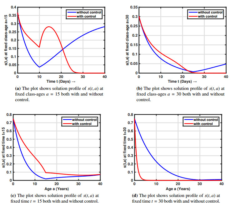
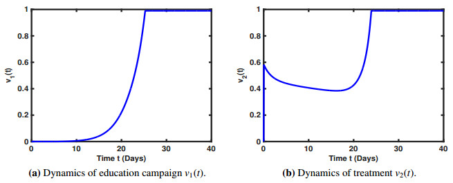
In the present manuscript, an age-structured heroin epidemic model is formulated with the assumption that susceptibility and recovery are age-dependent. Keeping in view some control measures for heroin addiction, a control problem for further analysis is presented. The main results are the existence of control variables, sensitivities, adjoint system and the setting of an optimal control problem. We used the techniques of weak derivatives and a general principle of Pontryagin's type for obtaining the optimal control problem. To compare our results, we demonstrated sample simulations which show the effect of control on the entire population.
- heroin epidemics,
- age-structure,
- control theory,
- weak derivatives,
- adjoint equations
Citation: Asaf Khan, Gul Zaman, Roman Ullah, Nawazish Naveed. Optimal control strategies for a heroin epidemic model with age-dependent susceptibility and recovery-age[J]. AIMS Mathematics, 2021, 6(2): 1377-1394. doi: 10.3934/math.2021086

Related Papers:

Abstract

In the present manuscript, an age-structured heroin epidemic model is formulated with the assumption that susceptibility and recovery are age-dependent. Keeping in view some control measures for heroin addiction, a control problem for further analysis is presented. The main results are the existence of control variables, sensitivities, adjoint system and the setting of an optimal control problem. We used the techniques of weak derivatives and a general principle of Pontryagin's type for obtaining the optimal control problem. To compare our results, we demonstrated sample simulations which show the effect of control on the entire population.

References

[1]	NIDA, Heroin, National Institute on Drug Abuse, 27 June 2019. Available from: https: //www.drugabuse.gov/publications/drugfacts/heroin.
[2]	Today's Heroin Epidemic, Center for Disease Control and Prevention (CDC), July 2015.
[3]	M. Iannelli, Mathematical Theory of Age-Structured Population Dynamics, Giardini Editori e Stampatori, Pisa, 1994.
[4]	H. R. Thieme, Mathematics in Populations Biology, Princeton University Press, Princeton, 2003.
[5]	H. R. Thieme, C. Castillo-Chavez, How many infection-age-dependent infectivity affect the dynamics of HIV/AIDS?, SIAM J. Appl. Math., 53 (2014), 14-47.
[6]	S. P. Rajasekar, M. Pitchaimani, Quanxin Zhu, Dynamic threshold probe of stochastic SIR model with saturated incidence rate and saturated treatment function, Physica A: Statistical Mechanics and its Applications, 535 (2019), 122300.
[7]	G. Zamana, Y. Saitob, M. Khanc, Optimal vaccination of an endemic model with variable infectivity and infinite delay, Zeitschrift für Naturforschung A, 68 (2013), 677-685.
[8]	M. Ma, S. Liu, J. Li, Bifurcation of a heroin model with nonlinear incidence rate, Nonlinear Dyn., 88 (2017), 555-565. doi: 10.1007/s11071-016-3260-9
[9]	G. P. Samanta, Dynamic behaviour for a nonautonomous heroin epidemic model with time delay, J. Appl. Math. Comput., 35 (2011), 161-178. doi: 10.1007/s12190-009-0349-z
[10]	I. M. Wangari, L. Stone, Analysis of a heroin epidemic model with saturated treatment function, J. Appl. Math., 2017 (2017), 1-22.
[11]	J. Liu, T. Zhang, Global behaviour of a heroin epidemic model with distributed delays, Appl. Math. Lett., 24 (2011), 1685-1692. doi: 10.1016/j.aml.2011.04.019
[12]	B. Fang, X. Li, M. Martcheva, L. Cai, Global asymptotic properties of a heroin epidemic model with treat-age, Appl. Math. Comput., 263 (2015), 315-331.
[13]	S. Djilali, T. M. Touaoula, S. E. H. Miri, A heroin epidemic model: very general non linear incidence, treat-age, and global stability, Acta Appl. Math., 152 (2017), 171-194.
[14]	E. White, C. Comiskey, Heroin epidemics, treatment and ODE modelling, Math. Biosci., 208 (2007), 312-324.
[15]	G. Mulone, B. Straughan, A note on heroin epidemics, Math. Biosci., 218 (2009), 138-141.
[16]	J. Mushanyu, F. Nyabadza, G. Muchatibaya, A. G. R. Stewart, Modelling multiple relapses in drug epidemics, Ricerche Mat., 65 (2016), 37-63. doi: 10.1007/s11587-015-0241-0
[17]	B. Fang, X. Li, M. Martcheva, L. Cai, Global stability for a heroin model with two distributed delays, Disc. Cont. Dyna. Sys., 19 (2014), 715-733.
[18]	Y. Muroya, H. Li, T. Kuniya, Complete global analysis of an SIRS epidemic model with graded cure and incomplete recovery rates, J. Math. Anal. Appl., 410 (2014), 719-732. doi: 10.1016/j.jmaa.2013.08.024
[19]	F. Nyabadza, S. D. Hove-Musekwa, From heroin epidemics to methamphetamine epidemics: Modelling substance abuse in a South African province, Math. Biosci., 225 (2010), 132-140.
[20]	G. Huang, A. Liu, A note on global stability for a heroin epidemic model with distributed delay, Appl. Math. Lett., 26 (2013), 687-691. doi: 10.1016/j.aml.2013.01.010
[21]	X. Liu, J. Wang, Epidemic dynamics on a delayed multi-group heroin epidemic model with nonlinear incidence rate, J. Nonlinear Sci. Appl., 9 (2016), 2149-2160. doi: 10.22436/jnsa.009.05.20
[22]	B. Fang, X. Li, M. Martcheva, L. Cai, Global stability for a heroin model with age-dependent susceptibility, J. Syst. Sci. Complex., 28 (2015), 1243-1257. doi: 10.1007/s11424-015-3243-9
[23]	J. Yang, X. Li, F. Zhang, Global dynamics of a heroin epidemic model with age structure and nonlinear incidence, Int. J. Biomath., 9 (2016), 1650033. doi: 10.1142/S1793524516500339
[24]	J. Wang, J. Wang, T. Kuniya, Analysis of an age-structured multi-group heroin epidemic model, Appl. Math. Comput., 347 (2019), 78-100.
[25]	G. Grippenberg, S. O. Londen, O. Staffans, Volterra Integral and Functional Equations, Cambridge University Press, Cambridge, 1990.
[26]	G. F. Webb, Theory of Nonlinear Age-dependent Population Dynamics, Marcel Dekker: New York, 1985.
[27]	X. Li, J. Yong, Optimal Control Theory for Infinite Dimensional Systems, Birkhäuser: Boston, 1995.
[28]	A. Khan, G. Zaman, Optimal control strategy of SEIR endemic model with continuous agestructure in the exposed and infectious classes, Optim. Contr. Appl. Meth., 39 (2018), 1716-1727. doi: 10.1002/oca.2437
[29]	D. L. Lukes, Differential Equations: Classical to Controlled, Mathematics in Science and Engineering, Academic Press: New York, 1982.
[30]	M. Martcheva, Age-Structured Epidemic Models. In: An Introduction to Mathematical Epidemiology, Texts in Applied Mathematics, Vol 61, Springer, Boston, MA, 2015.
[31]	M. Thater, K. Chudej, H. J. Pesch, Optimal vaccination strategies for an SEIR model of infectious diseases with logistic growth, Math. Biosc. Eng., 15 (2017), 485-505. doi: 10.3934/mbe.2018022

Reader Comments

Your name:*

Email:*
© 2021 the Author(s), licensee AIMS Press. This is an open access article distributed under the terms of the Creative Commons Attribution License (http://creativecommons.org/licenses/by/4.0)