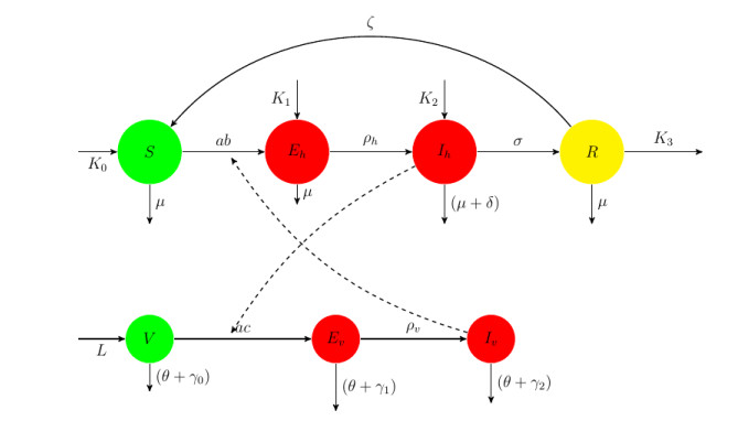
We present a compartmental model in ordinary differential equations of malaria disease transmission, accommodating the effect of indoor residual spraying on the vector population. The model allows for influx of infected migrants into the host population and for outflow of recovered migrants. The system is shown to have positive solutions. In the special case of no infected immigrants, we prove global stability of the disease-free equilibrium. Existence of a unique endemic equilibrium point is also established for the case of positive influx of infected migrants. As a case study we consider the combined South African malaria region. Using data covering 31 years, we quantify the effect of malaria infected immigrants on the South African malaria region.
Citation: Peter Witbooi, Gbenga Abiodun, Mozart Nsuami. A model of malaria population dynamics with migrants[J]. Mathematical Biosciences and Engineering, 2021, 18(6): 7301-7317. doi: 10.3934/mbe.2021361
We present a compartmental model in ordinary differential equations of malaria disease transmission, accommodating the effect of indoor residual spraying on the vector population. The model allows for influx of infected migrants into the host population and for outflow of recovered migrants. The system is shown to have positive solutions. In the special case of no infected immigrants, we prove global stability of the disease-free equilibrium. Existence of a unique endemic equilibrium point is also established for the case of positive influx of infected migrants. As a case study we consider the combined South African malaria region. Using data covering 31 years, we quantify the effect of malaria infected immigrants on the South African malaria region.

| [1] | World Health Organization, 2015. Global technical strategy for malaria 2016–2030, Available from: http://www.who.int/malaria/publications/atoz/9789241564991/en/. |
| [2] |
N. Chitnis, A. Schapira, C. Schindler, M. A. Penny, T. A. Smith, Mathematical analysis to prioritise strategies for malaria elimination, J. Theor. Biol., 455 (2018), 118–130. doi: 10.1016/j.jtbi.2018.07.007

|
| [3] |
N. Chitnis, J. M. Hyman, J. M. Cushing, Determining important parameters in the spread of malaria through the sensitivity analysis of a mathematical model, Bull. Math. Bio., 70 (2008), 1272–1296. doi: 10.1007/s11538-008-9299-0
|
| [4] |
C. N. Ngonghala, M. I. Teboh-Ewungkem, G. A. Ngwa, Persistent oscillations and backward bifurcation in a malaria model with varying human and mosquito populations: implications for control, J. Math. Biol., 70 (2015), 1581–1622. doi: 10.1007/s00285-014-0804-9
|
| [5] |
G. A. Ngwa, W. S. Shu, A mathematical model for endemic malaria with variable human and mosquito populations, Math. Comput. Modelling, 32 (2000), 747–763. doi: 10.1016/S0895-7177(00)00169-2
|
| [6] |
I. Enahoro, S. Eikenberry, A. B. Gumel, S. Huijben, K. Paaijmans, Long-lasting insecticidal nets and the quest for malaria eradication: a mathematical modeling approach, J. Math. Biol., 81 (2020), 113–158. doi: 10.1007/s00285-020-01503-z
|
| [7] |
G. J. Abiodun, O. S. Makinde, A. M. Adeola, K. Y. Njabo, P. J. Witbooi, R. Djidjou-Demasse, et al., A Dynamical and Zero-Inflated Negative Binomial Regression Modelling of Malaria Incidence in Limpopo Province, South Africa, Int. J. Environ. Res. Public Health, 16 (2019), 2000. doi: 10.3390/ijerph16112000
|
| [8] | F. B. Agusto, N. Marcus, K. O. Okosun, Application of optimal control to the epidemiology of malaria, Electron. J. Differ. Equ., 81 (2012), 1–22. |
| [9] | G. J. Abiodun, P. Witbooi, K. O. Okosun, Modelling the impact of climatic variables on malaria transmission, Hacettepe J. Math. Stat., 47 (2018), 219–235. |
| [10] | M. Arquam, A. Singh, H. Cherifi, Impact of Seasonal Conditions on Vector-Borne Epidemiological Dynamics, IEEE Access, 8 (2020), 94510–94525. |
| [11] | P. J. Witbooi, An SEIR model with infected immigrants and recovered emigrants, Adv. Differ. Equ., 1, (2021) 1–15. |
| [12] | L. F. Lopez, M. Amaku, F. Antonio, B. Coutinho, M. Quam, M. N. Burattini, et al., Modeling Importations and Exportations of Infectious Diseases via Travelers, Bull. Math. Biol., 78 (2016), 185209. |
| [13] |
A. Traore, Analysis of a vector-borne disease model with human and vectors immigration, J. Appl. Math. Comput., 64 (2020), 411–428. doi: 10.1007/s12190-020-01361-4
|
| [14] |
B. Dembele, A. Yakubu, Controlling imported malaria cases in the United States of America, Math. Biosci. Eng., 14 (2017), 95–109. doi: 10.3934/mbe.2017007
|
| [15] |
M. A. Khan, E. Bonyah, Z. Hammouch, E. Mifta Shaiful, A mathematical model of tuberculosis (TB) transmission with children and adults groups: a fractional model, AIMS Math., 5 (2020), 2813–2842. doi: 10.3934/math.2020181
|
| [16] |
F. Brauer, P. van den Driessche, Models for transmission of disease with immigration of infectives, Math. Biosci., 171 (2001), 143–154. doi: 10.1016/S0025-5564(01)00057-8
|
| [17] | R. P. Sigdel, P. Ram, C. McCluskey, Global stability for an SEI model of infectious disease with immigration, Appl. Math. Comput., 243 (2014), 684–689. |
| [18] |
M. Coetzee, P. Kruger, R. H. Hunt, D. N. Durrheim, J. Urbach, C. F. Hansford, Malaria in South Africa: 110 years of learning to control the disease, S. Afr. Med. J., 103 (2013), 770–778. doi: 10.7196/SAMJ.7446
|
| [19] |
P. van den Driessche, J. Watmough, Reproduction numbers and sub-threshold endemic equilibria for compartmental models of disease transmission, Math. Biosci., 180 (2002), 29–48. doi: 10.1016/S0025-5564(02)00108-6
|
| [20] | X. Mao, Stochastic Differential Equations and Applications, Horwood, Chichester, 1997. |
| [21] |
E. Tornatore, P. Vetro, S. M. Buccellato, SIVR epidemic model with stochastic perturbation, Neural Comput. Appl., 24 (2014), 309–315. doi: 10.1007/s00521-012-1225-6
|
| [22] | G. J. Abiodun, B. O. Adebiyi, R. O. Abiodun, O. Oladimeji, K. E. Oladimeji, A. M. Adeola, et al., Investigating the resurgence of malaria prevalence in South Africa between 2015 and 2018: A scoping review, Open Public Health J., 13 (2020), 119125. |
| [23] | R. Maharaj, J. Raman, N. Morris, D. Moonasar, D. N. Durrheim, I. Seocharan, et al., Epidemiology of malaria in South Africa from control to elimination, S. Afr. Med. J., 203 (2013), 779–783. |
| [24] | P. J. Witbooi, G. J. Abiodun, G. J. van Schalkwyk, I. H. I. Ahmed, Stochastic modeling of a mosquito-borne disease, Adv. Differ. Equ., 1 (2020), 1–15. |
| [25] | World malaria report 2020. WHO. 2020 https://www.who.int/teams/global-malaria-programme/reports/world-malaria-report-2020/ |
| [26] | P. M. Mwamtobe, S. Abelman, J. M. Tchuenche, A. Kasambara, Optimal control of intervention strategies for malaria epidemic in Karonga District, Malawi, Abstr. Appl. Anal., 30 (2014), ID 594256. |
| [27] | G. Otieno, J. K. Koske, J. M. Mutiso, Transmission Dynamics and Optimal Control of Malaria in Kenya, Discrete Dyn. Nat. Soc., (2016), 8013574. |
| [28] |
J. A. N. Filipe, E. M. Riley, C. J. Drakeley, C. J. Sutherland, A. C. Ghani, Determination of the processes driving the acquisition of immunity to malaria using a mathematical transmission model, PLoS Comput. Biol., 3 (2007), e255. doi: 10.1371/journal.pcbi.0030255
|
| [29] | Worldometer, South Africa Population (2021), available from: https://www.worldometers.info/world-population/south-africa-population/. |
Figures(5) / Tables(3)

Peter Witbooi, Gbenga Abiodun, Mozart Nsuami. A model of malaria population dynamics with migrants[J]. Mathematical Biosciences and Engineering, 2021, 18(6): 7301-7317. doi: 10.3934/mbe.2021361


 DownLoad: