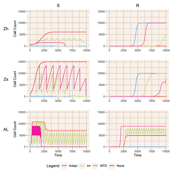
When eradication is impossible, cancer treatment aims to delay the emergence of resistance while minimizing cancer burden and treatment. Adaptive therapies may achieve these aims, with success based on three assumptions: resistance is costly, sensitive cells compete with resistant cells, and therapy reduces the population of sensitive cells. We use a range of mathematical models and treatment strategies to investigate the tradeoff between controlling cell populations and delaying the emergence of resistance. These models extend game theoretic and competition models with four additional components: 1) an Allee effect where cell populations grow more slowly at low population sizes, 2) healthy cells that compete with cancer cells, 3) immune cells that suppress cancer cells, and 4) resource competition for a growth factor like androgen. In comparing maximum tolerable dose, intermittent treatment, and adaptive therapy strategies, no therapeutic choice robustly breaks the three-way tradeoff among the three therapeutic aims. Almost all models show a tight tradeoff between time to emergence of resistant cells and cancer cell burden, with intermittent and adaptive therapies following identical curves. For most models, some adaptive therapies delay overall tumor growth more than intermittent therapies, but at the cost of higher cell populations. The Allee effect breaks these relationships, with some adaptive therapies performing poorly due to their failure to treat sufficiently to drive populations below the threshold. When eradication is impossible, no treatment can simultaneously delay emergence of resistance, limit total cancer cell numbers, and minimize treatment. Simple mathematical models can play a role in designing the next generation of therapies that balance these competing objectives.
Citation: Cassidy K. Buhler, Rebecca S. Terry, Kathryn G. Link, Frederick R. Adler. Do mechanisms matter? Comparing cancer treatment strategies across mathematical models and outcome objectives[J]. Mathematical Biosciences and Engineering, 2021, 18(5): 6305-6327. doi: 10.3934/mbe.2021315
When eradication is impossible, cancer treatment aims to delay the emergence of resistance while minimizing cancer burden and treatment. Adaptive therapies may achieve these aims, with success based on three assumptions: resistance is costly, sensitive cells compete with resistant cells, and therapy reduces the population of sensitive cells. We use a range of mathematical models and treatment strategies to investigate the tradeoff between controlling cell populations and delaying the emergence of resistance. These models extend game theoretic and competition models with four additional components: 1) an Allee effect where cell populations grow more slowly at low population sizes, 2) healthy cells that compete with cancer cells, 3) immune cells that suppress cancer cells, and 4) resource competition for a growth factor like androgen. In comparing maximum tolerable dose, intermittent treatment, and adaptive therapy strategies, no therapeutic choice robustly breaks the three-way tradeoff among the three therapeutic aims. Almost all models show a tight tradeoff between time to emergence of resistant cells and cancer cell burden, with intermittent and adaptive therapies following identical curves. For most models, some adaptive therapies delay overall tumor growth more than intermittent therapies, but at the cost of higher cell populations. The Allee effect breaks these relationships, with some adaptive therapies performing poorly due to their failure to treat sufficiently to drive populations below the threshold. When eradication is impossible, no treatment can simultaneously delay emergence of resistance, limit total cancer cell numbers, and minimize treatment. Simple mathematical models can play a role in designing the next generation of therapies that balance these competing objectives.

| [1] |
R. A. Gatenby, A change of strategy in the war on cancer, Nature, 459 (2009), 508–509. doi: 10.1038/459508a

|
| [2] |
R. A. Gatenby, J. Brown, T. Vincent, Lessons from applied ecology: Cancer control using an evolutionary double bind, Cancer Res., 69 (2009), 7499–7502. doi: 10.1158/0008-5472.CAN-09-1354
|
| [3] | R. A. Gatenby, A. S. Silva, R. J. Gillies, B. R. Frieden, Adaptive therapy, Cancer Res., 69 (2009), 4894–4903. |
| [4] |
K. L. Pogrebniak, C. Curtis, Harnessing tumor evolution to circumvent resistance, Trends Genet., 34 (2018), 639–651. doi: 10.1016/j.tig.2018.05.007
|
| [5] |
J. Zhang, J. J. Cunningham, J. S. Brown, R. A. Gatenby, Integrating evolutionary dynamics into treatment of metastatic castrate-resistant prostate cancer, Nat. Commun., 8 (2017), 1816. doi: 10.1038/s41467-017-01968-5
|
| [6] |
S. Benzekry, E. Pasquier, D. Barbolosi, B. Lacarelle, F. Barlési, N. André, J. Ciccolini, Metronomic reloaded: Theoretical models bringing chemotherapy into the era of precision medicine, Semin. Cancer Biol., 35 (2015), 53–61. doi: 10.1016/j.semcancer.2015.09.002
|
| [7] |
E. Hansen, A. F. Read, Modifying adaptive therapy to enhance competitive suppression, Cancers, 12 (2020), 3556. doi: 10.3390/cancers12123556
|
| [8] |
K. Akakura, N. Bruchovsky, S. L. Goldenberg, P. S. Rennie, A. R. Buckley, L. D. Sullivan, Effects of intermittent androgen suppression on androgen-dependent tumors. apoptosis and serum prostate-specific antigen, Cancer, 71 (1993), 2782–2790. doi: 10.1002/1097-0142(19930501)71:9<2782::AID-CNCR2820710916>3.0.CO;2-Z
|
| [9] | C. Simsek, E. Esin, S. Yalcin, Metronomic chemotherapy: A systematic review of the literature and clinical experience, J. Oncol., 2019 (2019), 1–31. |
| [10] |
A. Konstorum, T. Hillen, J. Lowengrub, Feedback regulation in a cancer stem cell model can cause an allee effect, Bull. Math. Biol., 78 (2016), 754–785. doi: 10.1007/s11538-016-0161-5
|
| [11] |
J. West, Y. Ma, P. K. Newton, Capitalizing on competition: An evolutionary model of competitive release in metastatic castration resistant prostate cancer treatment, J. Theor. Biol., 455 (2018), 249–260. doi: 10.1016/j.jtbi.2018.07.028
|
| [12] |
R. D. Holt, Predation, apparent competition and the structure of prey communities, Theor. Popul. Biol., 12 (1977), 197–229. doi: 10.1016/0040-5809(77)90042-9
|
| [13] |
E. Piretto, M. Delitala, M. Ferraro, Combination therapies and intra-tumoral competition: Insights from mathematical modeling, J. Theor. Biol., 446 (2018), 149–159. doi: 10.1016/j.jtbi.2018.03.014
|
| [14] |
H. Schättler, U. Ledzewicz, B. Amini, Dynamical properties of a minimally parameterized mathematical model for metronomic chemotherapy, J. Math. Biol., 72 (2016), 1255–1280. doi: 10.1007/s00285-015-0907-y
|
| [15] |
A. M. Ideta, G. Tanaka, T. Takeuchi, K. Aihara, A mathematical model of intermittent androgen suppression for prostate cancer, J. Nonlinear Sci., 18 (2008), 593. doi: 10.1007/s00332-008-9031-0
|
| [16] |
E. M. Rutter, Y. Kuang, Global dynamics of a model of joint hormone treatment with dendritic cell vaccine for prostate cancer, Discrete Contin. Dyn. Syst. B, 22 (2017), 1001–1021. doi: 10.3934/dcdsb.2017050
|
| [17] |
A. Zazoua, W. Wang, Analysis of mathematical model of prostate cancer with androgen deprivation therapy, Commun. Nonlinear Sci. Numer. Simul., 66 (2019), 41–60. doi: 10.1016/j.cnsns.2018.06.004
|
| [18] |
J. Baez, Y. Kuang, Mathematical models of androgen resistance in prostate cancer patients under intermittent androgen suppression therapy, Appl. Sci., 6 (2016), 352. doi: 10.3390/app6110352
|
| [19] |
H. V. Jain, S. K. Clinton, A. Bhinder, A. Friedman, Mathematical modeling of prostate cancer progression in response to androgen ablation therapy, Proc. Natl. Acad. Sci. USA, 108 (2011), 19701–19706. doi: 10.1073/pnas.1115750108
|
| [20] |
T. Portz, Y. Kuang, J. D. Nagy, A clinical data validated mathematical model of prostate cancer growth under intermittent androgen suppression therapy, AIP Adv., 2 (2012), 011002. doi: 10.1063/1.3697848
|
| [21] |
J. J. Cunningham, J. S. Brown, R. A. Gatenby, K. Staňková, Optimal control to develop therapeutic strategies for metastatic castrate resistant prostate cancer, J. Theor. Biol., 459 (2018), 67–78. doi: 10.1016/j.jtbi.2018.09.022
|
| [22] |
P. F. Sale, Maintenance of high diversity in coral reef fish communities, Am. Nat., 111 (1977), 337–359. doi: 10.1086/283164
|
| [23] |
R. A. Armstrong, R. McGehee, Competitive exclusion, Am. Nat., 115 (1980), 151–170. doi: 10.1086/283553
|
| [24] |
L. Schiffer, W. Arlt, K.-H. Storbeck, Intracrine androgen biosynthesis, metabolism and action revisited, Mol. Cell. Endocrinol., 465 (2018), 4–26. doi: 10.1016/j.mce.2017.08.016
|
| [25] |
Z. Zhu, Y.-M. Chung, O. Sergeeva, V. Kepe, M. Berk, J. Li, H.-K. Ko, Z. Li, M. Petro, F. P. DiFilippo et al., Loss of dihydrotestosterone-inactivation activity promotes prostate cancer castration resistance detectable by functional imaging, J. Biol. Chem., 293 (2018), 17829–17837. doi: 10.1074/jbc.RA118.004846
|
| [26] |
W. P. Harris, E. A. Mostaghel, P. S. Nelson, B. Montgomery, Androgen deprivation therapy: progress in understanding mechanisms of resistance and optimizing androgen depletion, Nat. Clin. Pract. Urol., 6 (2009), 76–85. doi: 10.1038/ncpuro1296
|
| [27] |
D. L. Suzman, E. S. Antonarakis, Does degree of androgen suppression matter in hormone-sensitive prostate cancer?, J. Clin. Oncol., 33 (2015), 1098–1100. doi: 10.1200/JCO.2014.60.1419
|
| [28] | K. E. Soetaert, T. Petzoldt, R. W. Setzer, Solving differential equations in R: package deSolve, J. Stat. Softw., 33 (2010), 1–25. |
| [29] |
K. Bacevic, R. Noble, A. Soffar, O. W. Ammar, B. Boszonyik, S. Prieto, C. Vincent, M. E. Hochberg, L. Krasinska, D. Fisher, Spatial competition constrains resistance to targeted cancer therapy, Nat. Commun., 8 (2017), 1995. doi: 10.1038/s41467-017-01516-1
|
| [30] |
J. A. Gallaher, P. M. Enriquez-Navas, K. A. Luddy, R. A. Gatenby, A. R. Anderson, Spatial heterogeneity and evolutionary dynamics modulate time to recurrence in continuous and adaptive cancer therapies, Cancer Res., 78 (2018), 2127–2139. doi: 10.1158/0008-5472.CAN-17-2649
|
| [31] |
A. B. Shah, K. A. Rejniak, J. L. Gevertz, Limiting the development of anti-cancer drug resistance in a spatial model of micrometastases, Math. Biosci. Eng., 13 (2016), 1185–1206. doi: 10.3934/mbe.2016038
|
| [32] |
M. S. Feizabadi, Modeling multi-mutation and drug resistance: analysis of some case studies, Theor. Biol. Med. Mod., 14 (2017), 6. doi: 10.1186/s12976-017-0052-y
|
| [33] |
Y. Hirata, N. Bruchovsky, K. Aihara, Development of a mathematical model that predicts the outcome of hormone therapy for prostate cancer, J. Theor. Biol., 264 (2010), 517–527. doi: 10.1016/j.jtbi.2010.02.027
|
| [34] |
R. Salgia, P. Kulkarni, The genetic/non-genetic duality of drug 'resistance'in cancer, Trends Cancer, 4 (2018), 110–118. doi: 10.1016/j.trecan.2018.01.001
|
| [35] |
J. West, P. K. Newton, Cellular interactions constrain tumor growth, Proc. Natl. Acad. Sci. USA, 116 (2019), 1918–1923. doi: 10.1073/pnas.1804150116
|
| [36] |
A. Ballesta, J. Clairambault, Physiologically based mathematical models to optimize therapies against metastatic colorectal cancer: a mini-review, Curr. Pharm. Design, 20 (2014), 37–48. doi: 10.2174/13816128113199990553
|
| [37] |
G. Aguadé-Gorgorió, R. Solé, Adaptive dynamics of unstable cancer populations: The canonical equation, Evol. Appl., 11 (2018), 1283–1292. doi: 10.1111/eva.12625
|
| [38] |
A. Arabameri, D. Asemani, J. Hadjati, A structural methodology for modeling immune-tumor interactions including pro-and anti-tumor factors for clinical applications, Math. Biosci., 304 (2018), 48–61. doi: 10.1016/j.mbs.2018.07.006
|
| [39] |
M. Robertson-Tessi, A. El-Kareh, A. Goriely, A mathematical model of tumor–immune interactions, J. Theor. Biol., 294 (2012), 56–73. doi: 10.1016/j.jtbi.2011.10.027
|
| [40] |
A. Lorz, T. Lorenzi, M. E. Hochberg, J. Clairambault, B. Perthame, Populational adaptive evolution, chemotherapeutic resistance and multiple anti-cancer therapies, ESAIM: Math. Model. Num., 47 (2013), 377–399. doi: 10.1051/m2an/2012031
|
| [41] |
A. S. Silva, R. A. Gatenby, A theoretical quantitative model for evolution of cancer chemotherapy resistance, Biol. Direct, 5 (2010), 25. doi: 10.1186/1745-6150-5-25
|
| [42] |
J. West, L. You, J. Zhang, R. A. Gatenby, J. S. Brown, P. K. Newton, A. R. Anderson, Towards multi-drug adaptive therapy, Cancer Res., 80 (2020), 1578–1589. doi: 10.1158/0008-5472.CAN-19-2669
|
| [43] |
J. B. West, M. N. Dinh, J. S. Brown, J. Zhang, A. R. Anderson, R. A. Gatenby, Multidrug cancer therapy in metastatic castrate-resistant prostate cancer: An evolution-based strategy, Clin. Cancer Res., 25 (2019), 4413–4421. doi: 10.1158/1078-0432.CCR-19-0006
|
| [44] | J. L. Gevertz, J. R. Wares, Developing a minimally structured mathematical model of cancer treatment with oncolytic viruses and dendritic cell injections, Comput. Math. Methods Med., 2018 (2018), 8760371. |
| [45] |
A. Kaznatcheev, J. Peacock, D. Basanta, A. Marusyk, J. G. Scott, Fibroblasts and Alectinib switch the evolutionary games played by non-small cell lung cancer, Nat. Ecol. Evol., 3 (2019), 450–456. doi: 10.1038/s41559-018-0768-z
|
| [46] | M. Gluzman, J. G. Scott, A. Vladimirsky, Optimizing adaptive cancer therapy: dynamic programming and evolutionary game theory, arXiv preprint arXiv: 1812.01805. |
| [47] |
Y. Hirata, K. Morino, K. Akakura, C. S. Higano, K. Aihara, Personalizing androgen suppression for prostate cancer using mathematical modeling, Sci. Rep., 8 (2018), 2673. doi: 10.1038/s41598-018-20788-1
|
| [48] |
Y. Viossat, R. Noble, A theoretical analysis of tumour containment, Nat. Ecol. Evol., 5 (2021), 826–835. doi: 10.1038/s41559-021-01428-w
|
| [49] |
F. F. Teles, J. M. Lemos, Cancer therapy optimization based on multiple model adaptive control, Biomed. Signal Process. Control, 48 (2019), 255–264. doi: 10.1016/j.bspc.2018.09.016
|
| [50] |
U. Ledzewicz, S. Wang, H. Schättler, N. André, M. A. Heng, E. Pasquier, On drug resistance and metronomic chemotherapy: A mathematical modeling and optimal control approach, Math. Biosci. Eng., 14 (2017), 217–235. doi: 10.3934/mbe.2017014
|
| [51] |
A. Alvarez-Arenas, K. E. Starkov, G. F. Calvo, J. Belmonte-Beitia, Ultimate dynamics and optimal control of a multi-compartment model of tumor resistance to chemotherapy, Discrete Contin. Dyn. Syst. B, 24 (2019), 2017–2038. doi: 10.3934/dcdsb.2019082
|
| [52] | C. Cockrell, D. E. Axelrod, Optimization of dose schedules for chemotherapy of early colon cancer determined by high-performance computer simulations, Cancer Inform., 18 (2019), 1176935118822804. |
| [53] | K. Normilio-Silva, A. C. de Figueiredo, A. C. Pedroso-de Lima, G. Tunes-da Silva, A. Nunes da Silva, A. Delgado Dias Levites, A. T. de Simone, P. Lopes Safra, R. Zancani, P. C. Tonini et al., Long-term survival, quality of life, and quality-adjusted survival in critically ill patients with cancer, Crit. Care Med., 44 (2016), 1327–1337. |
| [54] |
T. Hatano, Y. Hirata, H. Suzuki, K. Aihara, Comparison between mathematical models of intermittent androgen suppression for prostate cancer, J. Theor. Biol., 366 (2015), 33–45. doi: 10.1016/j.jtbi.2014.10.034
|
| [55] | J. I. Griffiths, P. Wallet, L. T. Pflieger, D. Stenehjem, X. Liu, P. A. Cosgrove, N. A. Leggett, J. A. McQuerry, G. Shrestha, M. Rosetti, G. Sunga, P. J. Moos, F. R. Adler, J. T. Chang, S. Sharma, A. Bild, Circulating immune cell phenotype dynamics reflect the strength of tumor-immune cell interactions in patients during immunotherapy, Proc. Natl. Acad. Sci. USA, in press. |
| [56] |
R. A. Beckman, G. S. Schemmann, C.-H. Yeang, Impact of genetic dynamics and single-cell heterogeneity on development of nonstandard personalized medicine strategies for cancer, Proc. Natl. Acad. Sci. USA, 109 (2012), 14586–14591. doi: 10.1073/pnas.1203559109
|
| [57] |
K. Staňková, J. S. Brown, W. S. Dalton, R. A. Gatenby, Optimizing cancer treatment using game theory: A review, JAMA Oncol., 5 (2019), 96–103. doi: 10.1001/jamaoncol.2018.3395
|

Figures(5) / Tables(2)

Cassidy K. Buhler, Rebecca S. Terry, Kathryn G. Link, Frederick R. Adler. Do mechanisms matter? Comparing cancer treatment strategies across mathematical models and outcome objectives[J]. Mathematical Biosciences and Engineering, 2021, 18(5): 6305-6327. doi: 10.3934/mbe.2021315


 DownLoad: