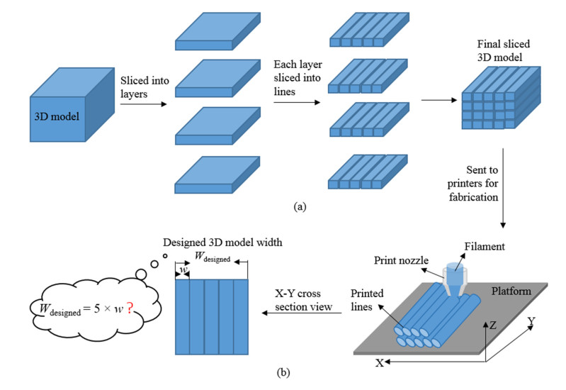
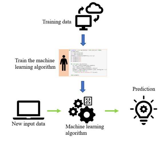
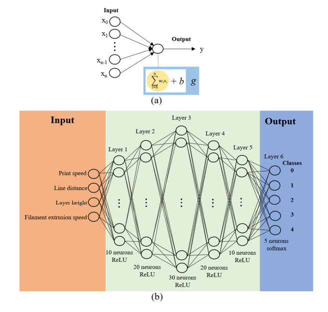
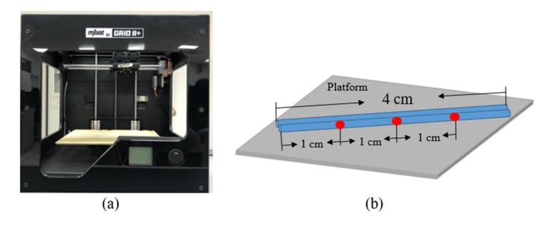
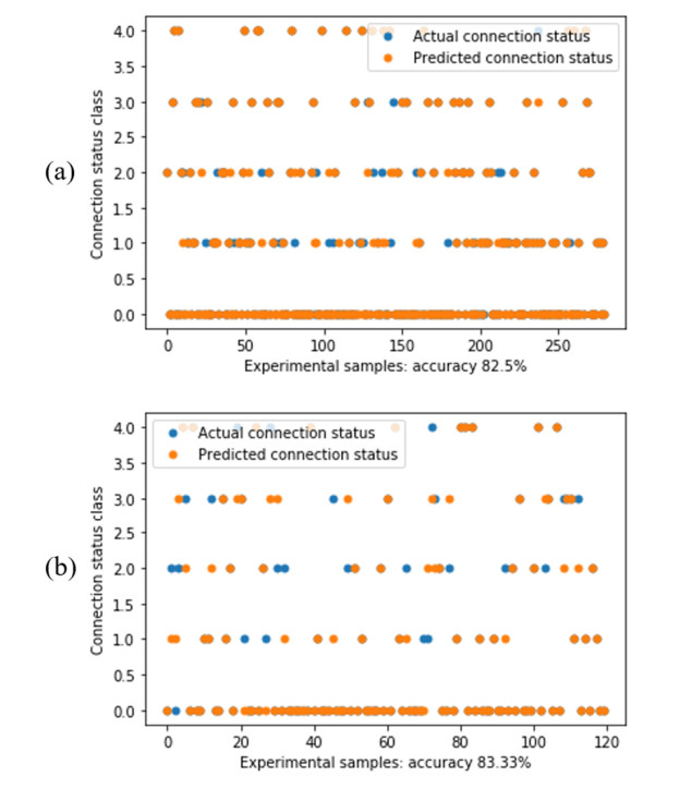
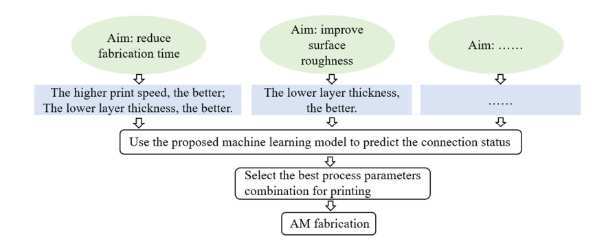
Additive manufacturing is becoming increasingly popular because of its unique advantages, especially fused deposition modelling (FDM) which has been widely used due to its simplicity and comparatively low price. All the process parameters of FDM can be changed to achieve different goals. For example, lower print speed may lead to higher strength of the fabricated parts. While changing these parameters (e.g. print speed, layer height, filament extrusion speed and path distance in a layer), the connection between paths (lines) in a layer will be changed. To achieve the best connection among paths in a real printing process, how these parameters may result in what kind of connection should be studied. In this paper, a machine learning (deep neural network) model is proposed to predict the connection between paths in different process parameters. Four hundred experiments were conducted on an FDM machine to obtain the corresponding connection status data. Among them, there are 280 groups of data that were used to train the machine learning model, while the rest 120 groups of data were used for testing. The results show that this machine learning model can predict the connection status with the accuracy of around 83%. In the future, this model can be used to select the best process parameters in additive manufacturing processes with corresponding objectives.
Citation: Jingchao Jiang, Chunling Yu, Xun Xu, Yongsheng Ma, Jikai Liu. Achieving better connections between deposited lines in additive manufacturing via machine learning[J]. Mathematical Biosciences and Engineering, 2020, 17(4): 3382-3394. doi: 10.3934/mbe.2020191
Additive manufacturing is becoming increasingly popular because of its unique advantages, especially fused deposition modelling (FDM) which has been widely used due to its simplicity and comparatively low price. All the process parameters of FDM can be changed to achieve different goals. For example, lower print speed may lead to higher strength of the fabricated parts. While changing these parameters (e.g. print speed, layer height, filament extrusion speed and path distance in a layer), the connection between paths (lines) in a layer will be changed. To achieve the best connection among paths in a real printing process, how these parameters may result in what kind of connection should be studied. In this paper, a machine learning (deep neural network) model is proposed to predict the connection between paths in different process parameters. Four hundred experiments were conducted on an FDM machine to obtain the corresponding connection status data. Among them, there are 280 groups of data that were used to train the machine learning model, while the rest 120 groups of data were used for testing. The results show that this machine learning model can predict the connection status with the accuracy of around 83%. In the future, this model can be used to select the best process parameters in additive manufacturing processes with corresponding objectives.

| [1] |
J. Liu, A. T. Gaynor, S. Chen, Z. Kang, K. Suresh, A. Takezawa, et al., Current and future trends in topology optimization for additive manufacturing, Struct. Multidiscip. Optim., 57 (2018), 2457-2483. doi: 10.1007/s00158-018-1994-3

|
| [2] |
J. Liu, Y. Zheng, R. Ahmad, J. Tang, Y. Ma, Minimum length scale constraints in multi-scale topology optimisation for additive manufacturing, Virtual. Phys. Prototyping, 14 (2019), 229-241. doi: 10.1080/17452759.2019.1584944
|
| [3] |
Y. F. Fu, B. Rolfe, L. N. S. Chiu, Y. Wang, X. Huang, K. Ghabraie, Design and experimental validation of self-supporting topologies for additive manufacturing, Virtual. Phys. Prototyping, 14 (2019), 382-394. doi: 10.1080/17452759.2019.1637023
|
| [4] |
H. Yu, J. Huang, B. Zou, W. Shao, J. Liu, Stress-constrained shell-lattice infill structural optimisation for additive manufacturing. Virtual. Phys. Prototyping, 15 (2020), 35-48. doi: 10.1080/17452759.2019.1647488
|
| [5] |
J. Liu, Piecewise length scale control for topology optimization with an irregular design domain, Comput. Methods Appl. Mech. Eng., 351 (2019), 744-765. doi: 10.1016/j.cma.2019.04.014
|
| [6] |
C. Wang, X. Tan, E. Liu, S. Tor, Process parameter optimization and mechanical properties for additively manufactured stainless steel 316L parts by selective electron beam melting, Mater. Des., 147 (2018), 157-166. doi: 10.1016/j.matdes.2018.03.035
|
| [7] |
Y. Tang, G. Dong, Q. Zhou, Y. Zhao, Lattice Structure Design and Optimization With Additive Manufacturing Constraints, IEEE Trans. Autom. Sci. Eng., 15 (2018), 1546-1562. doi: 10.1109/TASE.2017.2685643
|
| [8] | C. Yu, J. Jiang, A Perspective on Using Machine Learning in 3D Bioprinting, Int. J. Bioprint., 6 (2020), 94-101. |
| [9] |
J. Jiang, J. Stringer, X. Xu, Support Optimization for Flat Features via Path Planning in Additive Manufacturing, 3D Print. Addit. Manuf., 6 (2019), 171-179. doi: 10.1089/3dp.2017.0124
|
| [10] | J. Jiang, X. Xu, J. Stringer, Support Structures for Additive Manufacturing: A Review, J. Manuf. Mater. Process., 2 (2018), 64. |
| [11] | T. Wuest, D. Weimer, C. Irgens, K. D. Thoben, Machine learning in manufacturing: Advantages, challenges, and applications, Prod. Manuf. Res., 4 (2016), 23-45. |
| [12] | K. Aoyagi, H. Wang, H. Sudo, A. Chiba, Simple method to construct process maps for additive manufacturing using a support vector machine, Addit. Manuf., 27 (2019), 353-362. |
| [13] |
A. Menon, B. Póczos, A. W. Feinberg, N. R. Washbum, Optimization of Silicone 3D Printing with Hierarchical Machine Learning, 3D Print. Addit. Manuf., 6 (2019), 181-189. doi: 10.1089/3dp.2018.0088
|
| [14] |
H. He, Y. Yang, Y. Pan, Machine learning for continuous liquid interface production: Printing speed modelling, J. Manuf. Syst., 50 (2019), 236-246. doi: 10.1016/j.jmsy.2019.01.004
|
| [15] |
J. Francis, L. Bian, Deep Learning for Distortion Prediction in Laser-Based Additive Manufacturing using Big Data, Manuf. Lett., 20 (2019), 10-14. doi: 10.1016/j.mfglet.2019.02.001
|
| [16] |
M. Khanzadeh, P. Rao, R. Jafari-Marandi, B. K. Smith, M. A. Tschopp, L. Bian, Quantifying Geometric Accuracy with Unsupervised Machine Learning: Using Self-Organizing Map on Fused Filament Fabrication Additive Manufacturing Parts, J. Manuf. Sci. Eng., 140 (2018), 031011. doi: 10.1115/1.4038598
|
| [17] |
Z. Zhu, N. Anwer, Q. Huang, L. Mathieu, Machine learning in tolerancing for additive manufacturing, CIRP Ann., 67 (2018), 157-160. doi: 10.1016/j.cirp.2018.04.119
|
| [18] | B. Zhang, S. Liu, Y. C. Shin, In-Process monitoring of porosity during laser additive manufacturing process, Addit. Manuf., 28 (2019), 497-505. |
| [19] |
F. Tamburrino, S. Graziosi, M. Bordegoni, The influence of slicing parameters on the multi-material adhesion mechanisms of FDM printed parts: An exploratory study, Virtual Phys. Prototyping, 14 (2019), 316-322. doi: 10.1080/17452759.2019.1607758
|
| [20] |
J. Jiang, J. Stringer, X. Xu, R. Y. Zhong, Investigation of printable threshold overhang angle in extrusion-based additive manufacturing for reducing support waste, Int. J. Comput. Integr. Manuf., 31 (2018), 961-969. doi: 10.1080/0951192X.2018.1466398
|
| [21] |
J. Jiang, J. Lou, G. Hu, Effect of Support on Printed Properties in Fused Deposition Modelling Processes, Virtual Phys. Prototyping, 14 (2019), 308-315. doi: 10.1080/17452759.2019.1568835
|
| [22] |
J. Jiang, G. Hu, X. Li, X. Xu, P. Zhang, J. Stringer, Analysis and prediction of printable bridge length in fused deposition modelling based on back propagation neural network, Virtual Phys. Prototyping, 14 (2019), 253-266. doi: 10.1080/17452759.2019.1576010
|
| [23] | F. Weng, S. Gao, J. Jiang, J. Wang, P. Guo, A novel strategy to fabricate thin 316L stainless steel rods by continuous direct metal deposition in Z direction, Addit. Manuf., 27 (2019), 474-481. |
| [24] |
J. Jiang, F. Weng, S. Gao, J. Stringer, X. Xu, P. Guo, A Support Interface Method for Easy Part Removal in Direct Metal Deposition, Manuf. Lett., 20 (2019), 30-33. doi: 10.1016/j.mfglet.2019.04.002
|
| [25] | J. Jiang, X. Xu, J. Stringer, Effect of Extrusion Temperature on Printable Threshold Overhang in Additive Manufacturing, CIRP Conference on Manufacturing Systems, 2019. Available from: https://www.researchgate.net/publication/333259282_Effect_of_Extrusion_Temperature_on_Printable_Threshold_Overhang_in_Additive_Manufacturing. |
| [26] |
J. Jiang, X. Xu, J. Stringer, Optimisation of multi-part production in additive manufacturing for reducing support waste, Virtual Phys. Prototyping, 14 (2019), 219-228. doi: 10.1080/17452759.2019.1585555
|
| [27] |
J. Jiang, X. Xu, J. Stringer, Optimization of Process Planning for Reducing Material Waste in Extrusion Based Additive Manufacturing, Rob. Comput. Integr. Manuf., 59 (2019), 317-325. doi: 10.1016/j.rcim.2019.05.007
|
| [28] | J. Jiang, X. Xu, J. Stringer, A new support strategy for reducing waste in additive manufacturing, The 48th International Conference on Computers and Industrial Engineering (CIE 48), 2018. Available from: https://www.researchgate.net/profile/Jingchao_Jiang/publication/329999272_A_New_Support_Strategy_for_Reducing_Waste_in_Additive_Manufacturing/links/5c367bf492851c22a368bcad/A-New-Support-Strategy-for-Reducing-Waste-in-Additive-Manufacturing.pdf. |
| [29] |
T. H. Luu, C. Altenhofen, T. Ewald, A. Stork, D. Fellner, Efficient slicing of Catmull-Clark solids for 3D printed objects with functionally graded material, Comput. Graph, 82 (2019), 295-303. doi: 10.1016/j.cag.2019.05.023
|
| [30] |
Y. Wang, W. Li, A slicing algorithm to guarantee non-negative error of additive manufactured parts, Int. J. Adv. Manuf. Technol., 101 (2019), 3157-3166. doi: 10.1007/s00170-018-3199-8
|
| [31] |
J. Flores, I. Garmendia, J. Pujana, Toolpath generation for the manufacture of metallic components by means of the laser metal deposition technique, Int. J. Adv. Manuf. Technol., 101 (2019), 2111-2120. doi: 10.1007/s00170-018-3124-1
|
| [32] |
N. Volpato, T. T. Zanotto, Analysis of deposition sequence in tool-path optimization for low-cost material extrusion additive manufacturing, Int. J. Adv. Manuf. Technol., 101 (2019), 1855-1863. doi: 10.1007/s00170-018-3108-1
|
| [33] |
B. Ezair, S. Fuhrmann, G. Elber, Volumetric covering print-paths for additive manufacturing of 3D models, Comput. Aided Des., 100 (2018), 1-13. doi: 10.1016/j.cad.2018.02.006
|
| [34] |
Y. Xiong, S. I. Park, S. Padmanathan, A. G. Dharmawan, S. Foong, D. W. Rosen, et al., Process planning for adaptive contour parallel toolpath in additive manufacturing with variable bead width, Int. J. Adv. Manuf. Technol., 105 (2019), 4159-4170. doi: 10.1007/s00170-019-03954-1
|
| [35] |
B. Huang, W. Wang, S. Ren, R. Y. Zhong, J. Jiang, A proactive task dispatching method based on future bottleneck prediction for the smart factory, Int. J. Comput. Integr. Manuf., 32 (2019), 278-293. doi: 10.1080/0951192X.2019.1571241
|
| [36] | R. Caruana, A. Niculescu-Mizil, An empirical comparison of supervised learning algorithms, ACM International Conference Proceeding Series, 2006,161-168. Available from: https://dl.acm.org/doi/abs/10.1145/1143844.1143865. |
| [37] | L. Francis, Unsupervised learning, Predict. Model. Appl. Actuarial Sci., 1 (2014), 280-311. |
| [38] |
K. Arulkumaran, M. P. Deisenroth, M. Brundage, A. A. Bharath, Deep reinforcement learning: A brief survey, IEEE Signal Process. Mag., 34 (2017), 26-38. doi: 10.1109/MSP.2017.2743240
|
| [39] | K. He, X. Zhang, S. Ren, J. Sun, Delving Deep into Rectifiers: Surpassing Human-Level Performance on ImageNet Classification, The IEEE International Conference on Computer Vision (ICCV), 2015, 1026-1034. Available from: https://www.cv-foundation.org/openaccess/content_iccv_2015/html/He_Delving_Deep_into_ICCV_2015_paper.html. |
| [40] | D. P. Kingma, J. Ba, Adam: A method for stochastic optimization, arXiv: 1412.6980, 2017. |
| [41] |
J. M. Chacón, M. A. Caminero, E. García-Plaza, P. J. Núñez, Additive manufacturing of PLA structures using fused deposition modelling: Effect of process parameters on mechanical properties and their optimal selection, Mater. Des., 124 (2017), 143-157. doi: 10.1016/j.matdes.2017.03.065
|
| [42] |
A. Lanzotti, M. Grasso, G. Staiano, M. Martorelli, The impact of process parameters on mechanical properties of parts fabricated in PLA with an open-source 3-D printer, Rapid Prototyp J., 21 (2015), 604-617. doi: 10.1108/RPJ-09-2014-0135
|
| [43] | K. G. Christiyan, U. Chandrasekhar, K. Venkateswarlu, A study on the influence of process parameters on the Mechanical Properties of 3D printed ABS composite, IOP Conference Series: Materials Science and Engineering, Institute of Physics Publishing, 2016. Available from: https://iopscience.iop.org/article/10.1088/1757-899X/114/1/012109/meta. |
Figures(7) / Tables(3)

Jingchao Jiang, Chunling Yu, Xun Xu, Yongsheng Ma, Jikai Liu. Achieving better connections between deposited lines in additive manufacturing via machine learning[J]. Mathematical Biosciences and Engineering, 2020, 17(4): 3382-3394. doi: 10.3934/mbe.2020191


 DownLoad: