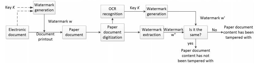
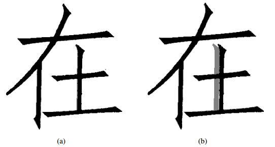
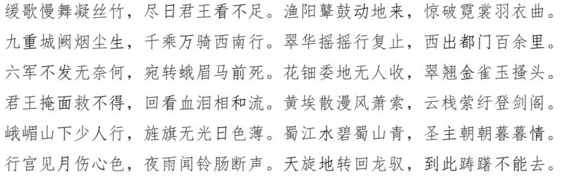
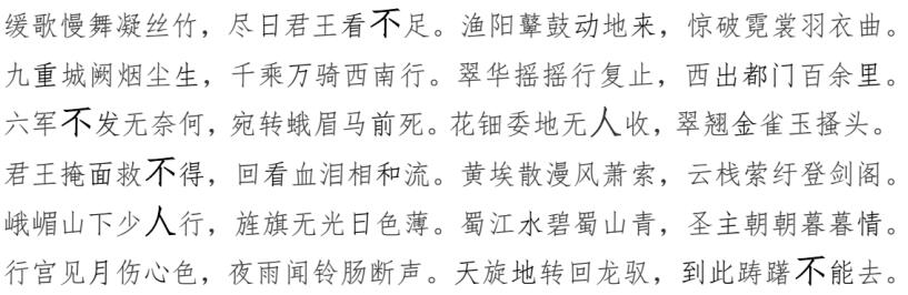
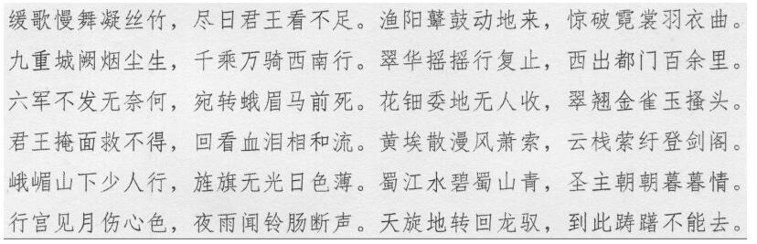
Aiming at the problem of easy tampering and difficult integrity authentication of paper text documents, this paper proposes a robust content authentication method for printed documents based on text watermarking scheme resisting print-and-scan attack. Firstly, an authentication watermark signal sequence related to content of text document is generated based on the Logistic chaotic map model; then, the authentication watermark signal sequence is embedded into printed paper document by using a robust text watermarking scheme; finally, the watermark information is extracted from scanned image of paper document, and compared with the authentication watermark information calculated in real time by the text document content obtained by OCR technology, thereby performing content integrity authentication of the paper text documents. Experimental results show that our method can achieve the robust content integrity authentication of paper text documents, and can also accurately locate the tampering position. In addition, the document after embedding the watermark information has a good visual effect, and the text watermarking scheme has a large information capacity.
Citation: Wenfa Qi, Wei Guo, Tong Zhang, Yuxin Liu, Zongming Guo, Xifeng Fang. Robust authentication for paper-based text documents based on text watermarking technology[J]. Mathematical Biosciences and Engineering, 2019, 16(4): 2233-2249. doi: 10.3934/mbe.2019110
Aiming at the problem of easy tampering and difficult integrity authentication of paper text documents, this paper proposes a robust content authentication method for printed documents based on text watermarking scheme resisting print-and-scan attack. Firstly, an authentication watermark signal sequence related to content of text document is generated based on the Logistic chaotic map model; then, the authentication watermark signal sequence is embedded into printed paper document by using a robust text watermarking scheme; finally, the watermark information is extracted from scanned image of paper document, and compared with the authentication watermark information calculated in real time by the text document content obtained by OCR technology, thereby performing content integrity authentication of the paper text documents. Experimental results show that our method can achieve the robust content integrity authentication of paper text documents, and can also accurately locate the tampering position. In addition, the document after embedding the watermark information has a good visual effect, and the text watermarking scheme has a large information capacity.

| [1] | J. Lee and C. S. Won, A watermarking sequence using parities of error control coding for image authentication and correction, IEEE Trans. Consum. Electron., 46 (2000), 313–317. |
| [2] | C. Li, Y. Wang and B. Ma, et al., Multi-block dependency based fragile watermarking scheme for fingerprint images protection, Multimed. Tools Appl., 64 (2013), 757–776. |
| [3] | X. Lv and Z. J. Wang, Perceptual image hashing based on shape contexts and local feature points, IEEE Trans. Inf. Forensics Security, 7 (2012), 1081–1093. |
| [4] | K. Maeno, Q. Sun and S. F. Chang, et al., New semi-fragile image authentication watermarking techniques using random bias and nonuniform quantization, IEEE Trans. Multimedia, 8 (2006), 32–45. |
| [5] | C. Qin, P. Ji and C. Chang, et al., Non-uniform Watermark Sharing Based on Optimal Iterative BTC for Image Tampering Recovery, IEEE Multimedia, 25 (2018), 36–48. |
| [6] | Z. Tang, X. Zhang and L. Huang, et al., Robust image hashing using ring-based entropies, Signal Process., 93 (2013), 2061–2069. |
| [7] | R. Vartak and S. Deshmukh, Survey of digital image authentication techniques, International Journal of Research in Advent Technology, 2 (2014), 176–179. |
| [8] | Y. Zhao, S. Wang and X. Zhang, et al., Robust hashing for image authentication using zernike moments and local features, IEEE Trans. Inf. Forensics Security, 8 (2013), 55–63. |
| [9] | Z. Yang, Y. Huang and X. Li, et al., Efficient secure data provenance scheme in multimedia outsourcing and sharing, CMC-Comput. Mat. Contin., 56 (2018), 1–17. |
| [10] | C. Qin, X. Chen and X. Luo, et al., Perceptual Image Hashing via Dual-cross Pattern Encoding and Salient Structure Detection, Inf. Sci., 423 (2018), 284–302. |
| [11] | J. Dittmann, A. Steinmetz and R. Steinmetz, Content-based digital signature for motion pictures authentication and content-fragile watermarking, in Proceedings IEEE International Conference on Multimedia Computing and Systems, IEEE, (1999), 209–213. |
| [12] | Z. Hou and X. Tang, Integrity authentication scheme of color video based on the fragile watermarking, in 2011 International Conference on Electronics, Communications and Control (ICECC), IEEE, (2011), 4354–4358. |
| [13] | T. S. Rao and R. R. Kurra, A smart intelligent way of video authentication using classification and decomposition of watermarking methods, preprint, arXiv: 1404.7237. |
| [14] | D. Xu, R. Wang and J. Wang, A novel watermarking scheme for H.264/AVC video authentication, Sig. Proc. Image Comm., 26 (2011), 267–279. |
| [15] | W. Zhang, Research on algorithm of digital video watermarking based on H.264 for copyright protection and content, Ph.D thesis, Beijing university of Post and telecommunications, 2013. |
| [16] | H. Zhu, The research of watermarking technology based on H.264/AVC, Ph.D thesis, Ningbo University, 2011. |
| [17] | J. Li, Digital watermarking technology for protecting the copyright of audio aggregation and authenticating the integrity of audio aggregation, Ph.D thesis, Ningbo University, 2012. |
| [18] | R. Wang and Y. Xiong, A novel watermarking algorithm for protecting audio aggregation based on ICA, in 6th International Conference on Digital Content, Multimedia Technology and its Applications, IEEE, (2010), 302–308. |
| [19] | X. Wang, P. Niu and M. Lu, A robust digital audio watermarking scheme using wavelet moment invariance, J. Syst. Softw., 84 (2011), 1408–1421. |
| [20] | I. K. Yeo and H. J. Kim, Modified patchwork algorithm: a novel audio watermarking scheme, IEEE Trans. Speech and Audio Processing, 11 (2003), 381–386. |
| [21] | Z. Jalil, A. M. Mirza and H. Jabeen, Word length based zero-watermarking algorithm for tamper detection in text documents, in 2010 2nd International Conference on Computer Engineering and Technology, IEEE, (2010), 376–378. |
| [22] | Q. C. Li and Z. H. Dong, Novel text watermarking algorithm based on chinese characters structure, in 2008 International Symposium on Computer Science and Computational Technology, IEEE, (2008), 348–351. |
| [23] | J. Liu, L. He and D. Fang, et al., A text digital watermarking for chinese word document, in 2008 International Symposium on Computer Science and Computational Technology, IEEE, (2008), 217–220. |
| [24] | L. Xiang, Y. Li and W. Hao, et al., Reversible natural language watermarking using synonym substitution and arithmetic coding, CMC-Comput. Mat. Contin., 55 (2018), 541–559. |
| [25] | L. Xiang, W. Wu and X. Li, et al., A linguistic steganography based on word indexing compression and candidate selection, Multimed. Tools Appl., 77 (2018), 28969–28989. |
| [26] | W. Guo, Y. Liu and B. Yang, et al., Research on information hiding technology in paper-based document, China Print. Pack. Study, 5 (2013), 30–34. |
| [27] | B. Yang, W. Shi and W. Qi, et al., Methods and apparatus for embedding and detecting digital watermarks in a text document, 2012, US Patent 8,107,129. |
| [28] | C. Ji, Y. Song and Z. Pang, A tamper proof method for the paper documents, 2012, China Patent 102,722,737. |
| [29] | T. Amano and D. Misaki, A feature calibration method for watermarking of document images, in Proceedings of the Fifth International Conference on Document Analysis and Recognition. ICDAR'99 (Cat. No. PR00318), IEEE, (1999), 91–94. |
| [30] | R. Chen, Research of Digital Watermarking technology to Resist Printing and Scanning, Ph.D thesis, Xidian University, 2014. |
| [31] | M. Lei, Y. Yang and R. Hu, A print resilient watermark scheme based on character complexity, J. B.J. Univer. Posts Telecom., 38 (2015), 58–62. |
| [32] | S. Li, A Study of Digital Watermarking Algorithm On Binary Text Image to Resist Hard-copy Attack, Ph.D thesis, Xidian University, 2012. |
| [33] | W. Qi, X. Li and B. Yang, et al., Document watermarking scheme for information tracking, J. Communicat., 29 (2008), 183–190. |
| [34] | M. Wu and B. Liu, Data hiding in binary image for authentication and annotation, IEEE Trans. Multimedia, 6 (2004), 528–538. |
| [35] | H. Yang and A. C. Kot, Pattern-based data hiding for binary image authentication by connectivity-preserving, IEEE Trans. Multimedia, 9 (2007), 475–486. |
| [36] | L. Xiang, J. Yu and C. Yang, et al., A word-embedding-based steganalysis method for linguistic steganography via synonym-substitution, IEEE Access, 6 (2018), 64131–64141. |
| [37] | S. Chen and H. Leung, Ergodic chaotic parameter modulation with application to digital image watermarking, IEEE Trans. Image Process., 14 (2005), 1590–1602. |
| [38] | Z. Li, Image authentication based on Digital Watermarking and Its Key Issues, Ph.D thesis, Beijing Jiaotong University, 2008. |
| [39] | G. Shao and M. Zhang, Novel fragile authentication watermark based on chaotic system, in 2004 IEEE International Symposium on Industrial Electronics, IEEE, (2004), 1491–1494. |
| [40] | J. C. Yoo and T. H. Han, Fast normalized cross-correlation, Circuits Syst. Signal Process., 28 (2009), 819–843. |
| [41] | Y. Niu and C. Zhang, Comparison of string similarity algorithm, Comput. Digit. Eng., 40 (2012), 14–17. |
| [42] | D. Liu, Research on novel text digital watermarking technologies and their typical applications, Ph.D thesis, University of Electronic Science and Technology, 2007. |
| [43] | Y. Liu, W. Guo and W. Qi, Researches on Text Image Watermarking Scheme Based on the Structure of Character Glyph, App. Mechan. Material., 731 (2015), 1163–1168. |


Figures(14) / Tables(1)

Wenfa Qi, Wei Guo, Tong Zhang, Yuxin Liu, Zongming Guo, Xifeng Fang. Robust authentication for paper-based text documents based on text watermarking technology[J]. Mathematical Biosciences and Engineering, 2019, 16(4): 2233-2249. doi: 10.3934/mbe.2019110


 DownLoad: