Low distortion reversible database watermarking based on hybrid intelligent algorithm

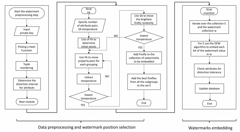
1.   Introduction

Differential equations play a very important role in modeling physical and engineering problems such as classical mechanics, thermodynamics, general relativity, and electro mechanics. From a broader perspective, the initial conditions are considered to be precisely defined in the model. There are uncertain errors in the observed, measured, or experimental data, which can be ambiguous, incomplete, or inaccurate. We can use the fuzzy differential equation (FDE) to overcome this uncertainty or inaccuracy. Fuzzy set theory was first introduced by Zadeh ^[1] which deals with uncertainty and vagueness. This theory has many applications in the study of artificial intelligence, decision making problems, soft computing, engineering and operation research. Differential equations play a significant role in modeling virtually every physical, technical, or biological process. Differential equations such as those used to solve real-life problems may not necessarily be directly solvable, that is, they do not have closed form solution. Instead, solution can be approximated using numerical methods. Every differential equation does not possess an exact solution. To overcome this situation, fuzzy set theory is a vital tool to deal with differential equations that do not possess exact solution due to uncertainty in their data. The initial conditions actually are the measurements or observations which lead to the vague information that is why, we use fuzzy differential equations to analyze this unclear information.

FODE may be viewed as a type of uncertain differential equation in which the uncertain values of parameters, coefficients, initial or boundary conditions are taken into account as fuzzy numbers. FODE has a worth buying significance from both practical and theoretical point of view. Chang and Zadeh ^[2] first introduced the idea of fuzzy derivative in 1972. The concept developed by Chang and Zadeh was followed up by Dubois and Prade ^[3], who used the theory of Zadeh's extension principle. FDEs were first discussed by Kaleva ^[4,5]. Bede and Gal ^[6] had defined strongly generalized Hukuhara differentiability (SGH-differentiability) of fuzzy-valued function. Kaleva discussed FDE using Puri-Relescue Hukuhara differentiability (H-differentiability) ^[6,7,8], gave the existence and uniqueness theorem for a solution of the FDE that satisfies the Lipschitz condition. Seikkala ^[9] introduced the fuzzy derivative which was the generalization of Hukuhara derivative, developed on the basis of Hukuhara difference (H-difference) ^[10]. Song and Wu ^[11] studied FDE, and they gave the generalization of the main consequences of Kaleva. FDE and fuzzy initial value problem (FIVP) were discussed by Kaleva in ^[12]. The derivative of a fuzzy-valued function can be evaluated using H-differentiability introduced by Hukuhara. Fuzzy set theory has great importance in solving FODEs. Many researchers ^{[13,14,15,16]} have established different techniques for solving FDEs and fuzzy linear systems. Allahviranloo et al. ^[17] introduced a method for solving fuzzy differential equation by Taylor expansion. Allahviranloo et al. ^[18] discussed the existence and uniqueness of the solution for the second-order FODE. Allahviranloo et al. ^[19] gave the numerical approach to solve FDEs using predictor-corrector method. Friedman et al. ^[20] gave the numerical approach to extract the solution of fuzzy differential equations and fuzzy integral equations. Wu ^[21] studied about fuzzy Riemann integral and its numerical integration. Many research articles have been published discussing the solution of fuzzy differential equations using different techniques ^{[22,23,24,25,26]}. Allahviraoloo and Ahmadi ^[27] introduced the concept of the fuzzy Laplace transform (FLT) to solve FDE. Salahshour and Allahviranloo ^[28] discussed many applications of the fuzzy Laplace transform. The FLT is an important and reliable technique for solving FDE and FIVP. The FLT has the benefit that it solves FIVPs directly without first evaluating a complementary solution and particular solution to FIVP. The FLT converts the fuzzy problem into an algebraic problem which can be easily solved. The initial conditions of FIVP are in the parametric form that splits the problem into two equations. Furthermore, by applying the Laplace transform and the inverse Laplace transform, we are able to find the solution of FIVP. Optimization plays a vital role in a number of fields for the development of technology. Many researchers have discussed advanced optimization algorithms for decision making problems ^[29]. Moreover, many research articles have been published regarding the importance of advanced optimization algorithms, for instance, heuristics and metaheuristics for challenging decision problems. There are many different domains where advanced optimization algorithms have been applied as solution approaches, such as online learning, scheduling, multi-objective optimization, transportation, medicine, data classification, and others ^{[30,31,32,33,34,35]}.

This research paper presents a new analytical method for solving fuzzy initial value problem of fourth-order FODE using the fuzzy Laplace transform. To this end, we establish the fourth order derivative of fuzzy-valued function according to the type of differentiability. We present the relationship between the fourth-order derivative and the Laplace transform of FVF. Moreover, we presents an algorithm to find the solution of fourth-order FIVP. The effectiveness of the introduced method is illustrated by an example. Furthermore, we solved another example about the switching point. The solution of the FIVP possessed the Mittag-Leffler function ^[36]. We express the solution of FIVP through graphical point of view to visualize and support the theoretical results.

In short, the main content of this research article has the following perspectives:

● Solution of fourth-order fuzzy initial value problem using the Laplace operator.

● An important relationship between the Laplace transform of the FVF and its fourth-order derivative.

● An algorithm is presented to understand the steps required to solve FIVP.

● The validity of the introduced method is verified by an illustrative example.

● Another example is solved about switching points.

● Application of fourth-order FIVP in RL circuit.

● Representation of graphs to visualize and support the theoretical results.

The rest of the paper is designed as follows: Section $2$ contains the preliminary concepts. Section $3$ presents the fourth-order derivative of FVF and the relationship between the fourth-order derivative and Laplace transform of FVF. Section $4$ contains the framework of research methodology for solving fourth-order FIVP, and the characteristic theorem for the solution of fourth-order FIVP. Section $5$ presents supportive numerical examples and an application of fourth-order FIVP in RL circuit. Concluding remarks are given in Section $6$.

2.   Preliminaries

In this section, we recall some basic concepts require for this research paper.

Definition 2.1. ^[37] A fuzzy set (FS) $R_{F}$ in $X$ is an object of the form

where $\mu:X\rightarrow [0, 1]$ denotes the degree of membership of an element $\mathfrak{t} \in X$.

Definition 2.2. ^[37] A fuzzy number (FN) $u$ is a non-empty subset of $X$ with the rule of membership grade $\mu:X\rightarrow [0, 1]$. Firmly, $u$ is convex, that is,

Also, $u$ is normal because there exists $\mathfrak{t}\in X$ such that $\mu(\mathfrak{t}) = 1$.

Definition 2.3. ^[37] A triangular fuzzy number (TFN) $u$ is a subset of FN in $R$ with the following membership function:

where $a\leq b \leq c$ and a TFN is denoted by $u = (a, b, c)$.

Definition 2.4. ^[37] A parametric fuzzy number (PFN) $\mathfrak{u}$ is an ordered pair of the functions $\mathfrak{u}_{1}(\mathfrak{p})$ and $\mathfrak{u}_{2}(\mathfrak{p})$, $0\leq \mathfrak{p} \leq 1$ that satisfy the following requirements:

● $\mathfrak{u}_{1}(\mathfrak{p})$ is a bounded left continuous, non-decreasing function over $(0, 1]$ and right continuous at $0$,

● $\mathfrak{u}_{2}(\mathfrak{p})$ is a bounded left continuous, non-increasing function over $(0, 1]$ and right continuous at $0$,

● $\mathfrak{u}_{1}(\mathfrak{p}) \leq \mathfrak{u}_{2}(\mathfrak{p})$, $0 \leq \mathfrak{p} \leq1$.

The collection of all parametric fuzzy numbers (PFNs) $(\mathfrak{u}_{1}(\mathfrak{p}), \mathfrak{u}_{2}(\mathfrak{p}))$ with the operations of addition and scalar multiplication is denoted by $E^{1}$.

Definition 2.5. ^[10] let $u$ and $v$ be two fuzzy numbers. If there exists a fuzzy number $w$ such that $u = w \oplus v$, then $w$ is called H-difference of $u$ and $v$ and is denoted by $u \ominus_{H} v$.

Remark 2.1. Throughout this paper, we use the notation $\ominus$ for H-difference.

Definition 2.6. ^[10] Let $X$ be a subset of $R$. A FVF $\vartheta : X \rightarrow E^{1}$ is said to be H-differentiable at $\mathfrak{t}_{0}\in X$ if and only if there exists a fuzzy number $\vartheta^{'}(\mathfrak{t}_{0})\in E^{1}$ such that the limits

both exist and are equal to $\vartheta^{'}(\mathfrak{t}_{0})$. In this case, $\vartheta^{'}(\mathfrak{t}_{0})$ is called the H-derivative of $\vartheta$ at $\mathfrak{t}_{0}$. If $\vartheta$ is H-differentiable at any $\mathfrak{t} \in X$, we call $\vartheta$ is H-differentiable over $X$.

Definition 2.7. ^[10] Let $u, v\in E^1$ be two fuzzy numbers. If there exists a fuzzy number $w$ such that:

then $w$ is called the gH-difference of $u$ and $v$. In terms of $\mathfrak{p}$-level sets, gH-difference is defined as:

and if H-difference exists, then $u \ominus v = u \ominus_{gH} v$.

Bede and Gal ^[6] defined SGH-differentiability of fuzzy-valued function based on H-difference ^[10].

Definition 2.8. ^[10] Let $X$ be a subset of $R$. A FVF $\vartheta : X\rightarrow E^{1}$ is said to be SGH-differentiable at $\mathfrak{t}_{0}\in X$ and $\vartheta^{'}(\mathfrak{t}_{0})\in E^1$ if one of the following conditions is satisfied:

$\rm (ı)$ For every $\delta > 0,$ the expressions $\vartheta(\mathfrak{t}_{0}+\delta)\ominus\vartheta(\mathfrak{t}_{0})$ and $\vartheta(\mathfrak{t}_{0})\ominus\vartheta(\mathfrak{t}_{0}-\delta)$ both exist such that

$\rm (ıı)$ For every $\delta > 0,$ the expressions $\vartheta(\mathfrak{t}_{0})\ominus\vartheta(\mathfrak{t}_{0}+\delta)$ and $\vartheta(\mathfrak{t}_{0}-\delta)\ominus\vartheta(\mathfrak{t}_{0})$ both exist such that

Moreover, if $\vartheta$ is differentiable at each $\mathfrak{t}\in X$, then we say that $\vartheta$ is differentiable over $X$.

Definition 2.9. ^[36] The Mittag-Leffler function in two parameters $\xi, \eta$ is defined by the series expansion:

The Laplace transform of the Mittag-Leffler function $E_{\xi, \eta}(\mathfrak{t})$ is given by:

Definition 2.10. ($\mathfrak{p}-$cut form) ^[6] Suppose that a FVF $\vartheta: R\rightarrow E^1$ is denoted by:

for all $\mathfrak{p}$ belongs to unit closed interval $[0, 1]$ and $\mathfrak{t} \in R$.

The 1st and 2nd differentiability of a FVF $\vartheta$ is defined by:

● If $\vartheta$ is 1st differentiable ((ı)-differentiable), then the functions ${\vartheta}_{1(\mathfrak{p})}(\mathfrak{t})$ and ${\vartheta}_{2(\mathfrak{p})}(\mathfrak{t})$ are differentiable and defined as:

● If $\vartheta$ is 2nd differentiable ((ıı)-differentiable), then the functions ${\vartheta}_{1(\mathfrak{p})}(\mathfrak{t})$ and ${\vartheta}_{2(\mathfrak{p})}(\mathfrak{t})$ are differentiable and defined as:

Definition 2.11. ^[38] Suppose that a function $\vartheta$ and $\vartheta^{'}$ are differentiable FVFs. The FVF $\vartheta$ is denoted by $[\vartheta(\mathfrak{t})]^{\mathfrak{p}} = [\vartheta_{1(\mathfrak{p})}(\mathfrak{t}), \vartheta_{2(\mathfrak{p})}(\mathfrak{t})]$ for all $\mathfrak{p}$ belongs to unit closed interval $[0, 1]$.

$\rm(i)$ If $\vartheta^{'}$ is $(ı)$-differentiable, then the functions $\vartheta_{1(\mathfrak{p})}(\mathfrak{t})$ and $\vartheta_{2(\mathfrak{p})}(\mathfrak{t})$ are differentiable and

$\rm(ii)$ If $\vartheta^{'}$ is $(ıı)$-differentiable, then the functions $\vartheta_{1(\mathfrak{p})}(\mathfrak{t})$ and $\vartheta_{2(\mathfrak{p})}(\mathfrak{t})$ are differentiable and

Definition 2.12. ^[39] Suppose that a function $\vartheta$, $\vartheta^{'}$ and $\vartheta^{''}$ are differentiable FVFs. The function $\vartheta$ is denoted by $[\vartheta(\mathfrak{t})]^{\mathfrak{p}} = [\vartheta_{1(\mathfrak{p})}(\mathfrak{t}), \vartheta_{2(\mathfrak{p})}(\mathfrak{t})]$ for all $\mathfrak{p}$ belongs to unit closed interval $[0, 1]$.

$\rm(i)$ If $\vartheta^{''}$ is $(ı)$-differentiable, then the function $\vartheta_{1(\mathfrak{p})}(\mathfrak{t})$ and $\vartheta_{2(\mathfrak{p})}(\mathfrak{t})$ are differentiable and

$\rm(ii)$ If $\vartheta^{''}$ is $(ıı)$-differentiable, then the functions $\vartheta_{1(\mathfrak{p})}(\mathfrak{t})$ and $\vartheta_{2(\mathfrak{p})}(\mathfrak{t})$ are differentiable and

3.   Fourth-order derivative of fuzzy-valued function and its Laplace transform

In this section, we introduce the fourth-order derivative of fuzzy-valued function on the base of SGH-differentiability which is then the extension of solving first order linear fuzzy differential equation to fourth-order linear fuzzy differential equation.

Definition 3.1. On the base of SGH-differentiability, we have the following cases to determine the nature of fourth-order derivative of fuzzy-valued function $[\vartheta(\mathfrak{t})]^{\mathfrak{p}}$ and to compare the lower and upper FVFs ${\vartheta}_{1(\mathfrak{p})}(\mathfrak{t})$ and ${\vartheta}_{2(\mathfrak{p})}(\mathfrak{t})$ respectively according to their fourth-order derivatives. The behavior of fourth-order derivative of FVF $[\vartheta(\mathfrak{t})]^{\mathfrak{p}}$ is represented by Table 1.

Definition 3.2. ^[40] The points in an interval where fuzzy differentiability of type-$(ı)$ changes to type-$(ıı)$ and vice versa are called switching points.

Example 3.1. ^[40] The concept of switching point can be understand by the example of second-order derivative of FVF. Table 2 indicates about the switching points.

In this research article, we briefly discuss about switching points.

Table 2 shows that the fuzzy-valued function $\vartheta$ follows the same differentiability if there is no switch (cases $1$ and $4$) in increasing or decreasing nature of function or there are two switches (cases $2$ and $3$).

Definition 3.3. ^[27] Let $\vartheta(\mathfrak{t})$ be a continuous FVF. Assume that $e^{-r\mathfrak{t}}\vartheta(\mathfrak{t})$ is an improper fuzzy Riemann integrable on $[0, \infty)$, then the integral $\int_{0}^{\infty}e^{-r\mathfrak{t}}\vartheta(\mathfrak{t})d\mathfrak{t}$ is said to be the fuzzy Laplace transform of fuzzy-valued function $\vartheta$ and its symbolic representation is given by:

In $\mathfrak{p}-$cut form, Eq (3.1) takes the following form:

where, $L[\vartheta(\mathfrak{t})]$ is the classical notation of Laplace transform of crisp function $\vartheta(\mathfrak{t})$.

Theorem 3.1. ^[27] Let $\vartheta^{'}(\mathfrak{t})$ be an integrable FVF and $\vartheta(\mathfrak{t})$ be the primitive of $\vartheta^{'}(\mathfrak{t})$ on $[0, \infty)$. Then the Laplace transform of the FVF $\vartheta^{'}(\mathfrak{t})$ according to the type of differentiability is given by:

$\rm(a)$ If $\vartheta$ is $(ı)-$differentiable, then

$\rm(b)$ If $\vartheta$ is $(ıı)-$differentiable, then

Theorem 3.2. ^[27]Let $\vartheta(\mathfrak{t})$ and $\omega(\mathfrak{t})$ be the continuous FVFs and $a, b$ are real constants. Then

We discuss an important result concerning the relationship between Laplace transform of FVF and its fourth-order derivative in the following theorem.

Theorem 3.3. Let $\vartheta(\mathfrak{t})$ be a fuzzy-valued function such that $e^{-r\mathfrak{t}}\vartheta(\mathfrak{t})$, $e^{-r\mathfrak{t}}\vartheta^{'}(\mathfrak{t})$, $e^{-r\mathfrak{t}}\vartheta^{''}(\mathfrak{t})$, $e^{-r\mathfrak{t}}\vartheta^{'''}(\mathfrak{t})$ and $e^{-r\mathfrak{t}}\vartheta^{(iv)}(\mathfrak{t})$ exist, differentiable and Riemann integrable on $[0, \infty)$. Then we have the following cases:

$\rm 1)$ If $\vartheta(\mathfrak{t})$, $\vartheta^{'}(\mathfrak{t})$, $\vartheta^{''}(\mathfrak{t})$, $\vartheta^{'''}(\mathfrak{t})$ are $(ı)$-differentiable, then

$\rm 2)$ If $\vartheta(\mathfrak{t})$, $\vartheta^{'}(\mathfrak{t})$, $\vartheta^{''}(\mathfrak{t})$ are $(ı)$-differentiable and $\vartheta^{'''}(\mathfrak{t})$ is $(ıı)$-differentiable, then

$\rm 3)$ If $\vartheta(\mathfrak{t})$, $\vartheta^{'}(\mathfrak{t})$, $\vartheta^{'''}(\mathfrak{t})$ are $(ı)$-differentiable and $\vartheta^{''}(\mathfrak{t})$ is $(ıı)$-differentiable, then,

$\rm 4)$ If $\vartheta(\mathfrak{t})$, $\vartheta^{'}(\mathfrak{t})$ are $(ı)$-differentiable and $\vartheta^{''}(\mathfrak{t})$, $\vartheta^{'''}(\mathfrak{t})$ are $(ıı)$-differentiable, then

$\rm 5)$ If $\vartheta(\mathfrak{t})$, $\vartheta^{''}(\mathfrak{t})$, $\vartheta^{'''}(\mathfrak{t})$ are $(ı)$-differentiable and $\vartheta^{'}(\mathfrak{t})$ is $(ıı)$-differentiable, then

$\rm 6)$ If $\vartheta(\mathfrak{t})$, $\vartheta^{''}(\mathfrak{t})$ are $(ı)$-differentiable and $\vartheta^{'}(\mathfrak{t})$, $\vartheta^{'''}(\mathfrak{t})$ are $(ıı)$-differentiable, then

$\rm 7)$ If $\vartheta(\mathfrak{t})$ is $(ı)$-differentiable and $\vartheta^{'}(\mathfrak{t})$, $\vartheta^{''}(\mathfrak{t})$, $\vartheta^{'''}(\mathfrak{t})$ are $(ıı)$-differentiable, then

$\rm 8)$ If $\vartheta(\mathfrak{t})$, $\vartheta^{'''}(\mathfrak{t})$ are $(ı)$-differentiable and $\vartheta^{'}(\mathfrak{t})$, $\vartheta^{''}(\mathfrak{t})$ are $(ıı)$-differentiable, then

$\rm 9)$ If $\vartheta(\mathfrak{t})$ is $(ıı)$-differentiable and $\vartheta^{'}(\mathfrak{t})$, $\vartheta^{''}(\mathfrak{t})$, $\vartheta^{'''}(\mathfrak{t})$ are $(ı)$-differentiable, then

$\rm 10)$ If $\vartheta(\mathfrak{t})$, $\vartheta^{'}(\mathfrak{t})$, $\vartheta^{''}(\mathfrak{t})$, $\vartheta^{'''}(\mathfrak{t})$ are $(ıı)$-differentiable, then

$\rm 11)$ If $\vartheta(\mathfrak{t})$, $\vartheta^{''}(\mathfrak{t})$ are $(ıı)$-differentiable and $\vartheta^{'}(\mathfrak{t})$, $\vartheta^{'''}(\mathfrak{t})$ are $(ı)$-differentiable, then

$\rm 12)$ If $\vartheta(\mathfrak{t})$, $\vartheta^{'''}(\mathfrak{t})$ are $(ıı)$-differentiable and $\vartheta^{'}(\mathfrak{t})$, $\vartheta^{''}(\mathfrak{t})$ are $(ı)$-differentiable, then

$\rm 13)$ If $\vartheta(\mathfrak{t})$, $\vartheta^{'}(\mathfrak{t})$ are $(ıı)$-differentiable and $\vartheta^{''}(\mathfrak{t})$, $\vartheta^{'''}(\mathfrak{t})$ are $(ı)$-differentiable, then

$\rm 14)$ If $\vartheta(\mathfrak{t})$, $\vartheta^{'}(\mathfrak{t})$, $\vartheta^{'''}(\mathfrak{t})$ are $(ıı)$-differentiable and $\vartheta^{''}(\mathfrak{t})$ is $(ı)$-differentiable, then

$\rm 15)$ If $\vartheta(\mathfrak{t})$, $\vartheta^{'}(\mathfrak{t})$, $\vartheta^{''}(\mathfrak{t})$ are $(ıı)$-differentiable and $\vartheta^{'''}(\mathfrak{t})$ is $(ı)$-differentiable, then

$\rm 16)$ If $\vartheta(\mathfrak{t})$, $\vartheta^{''}(\mathfrak{t})$, $\vartheta^{'''}(\mathfrak{t})$ are $(ıı)$-differentiable and $\vartheta^{'}(\mathfrak{t})$ is $(ı)$-differentiable, then

Proof. We only prove $1)$, $2)$ and $3)$ here. The proof of remaining cases can be found in Appendix. $

$\rm 1)$ If $\vartheta(\mathfrak{t})$, $\vartheta^{'}(\mathfrak{t})$, $\vartheta^{''}(\mathfrak{t})$, $\vartheta^{'''}(\mathfrak{t})$ are $(ı)$-differentiable, then

Suppose that $\vartheta(\mathfrak{t})$, $\vartheta^{'}(\mathfrak{t})$, $\vartheta^{''}(\mathfrak{t})$, $\vartheta^{'''}(\mathfrak{t})$ are $(ı)$-differentiable, then from Theorem 3.1, it follows that:

System (3.5) implies that:

$\rm 2)$ If $\vartheta(\mathfrak{t})$, $\vartheta^{'}(\mathfrak{t})$, $\vartheta^{''}(\mathfrak{t})$ are $(ı)$-differentiable and $\vartheta^{'''}(\mathfrak{t})$ is $(ıı)$-differentiable, then

Assume that $\vartheta(\mathfrak{t})$, $\vartheta^{'}(\mathfrak{t})$, $\vartheta^{''}(\mathfrak{t})$ are $(ı)$-differentiable and $\vartheta^{'''}(\mathfrak{t})$ is $(ıı)$-differentiable, then from Theorem 3.1, we have:

By assembling the identities in system (3.6), we have:

$\rm 3)$ If $\vartheta(\mathfrak{t})$, $\vartheta^{'}(\mathfrak{t})$, $\vartheta^{'''}(\mathfrak{t})$ are $(ı)$-differentiable and $\vartheta^{''}(\mathfrak{t})$ is $(ıı)$-differentiable, then

Given that $\vartheta(\mathfrak{t})$, $\vartheta^{'}(\mathfrak{t})$, $\vartheta^{'''}(\mathfrak{t})$ are $(ı)$-differentiable and $\vartheta^{''}(\mathfrak{t})$ is $(ıı)$-differentiable, then Theorem 3.1 yields that:

System (3.7) gives:

4.   Framework of research methodology

In this section, we present the framework of research methodology or construction steps to solve the following fourth-order FIVP:

where $\mathtt{F}$ is a FVF which is linear with respect to lower and upper bounds $({\vartheta}_{1(\mathfrak{p})}(\mathfrak{t}), {\vartheta}_{2(\mathfrak{p})}(\mathfrak{t}))$ and $\vartheta(\mathfrak{t}) = \big({\vartheta}_{1(\mathfrak{p})} (\mathfrak{t}), {\vartheta}_{2(\mathfrak{p})}(\mathfrak{t})\big)$ is a fuzzy function with $\mathfrak{t}\geq0$ and $\mathfrak{p} \in [0, 1]$. The initial conditions $\vartheta(0)$, $\vartheta^{'}(0)$, $\vartheta^{''}(0)$ and $\vartheta^{'''}(0)$ are expressed in $\mathfrak{p}-$cut form.

Step 1. First, we apply the fuzzy Laplace transform to system (4.1)

Step 2. Then, we use Definition 3.1 and Theorem 3.3 for each case according to the type of differentiability. For instance,

$\rm(1)$ If $\vartheta(\mathfrak{t})$, $\vartheta^{'}(\mathfrak{t})$, $\vartheta^{''}(\mathfrak{t})$, $\vartheta^{'''}(\mathfrak{t})$ are $(ı)$-differentiable, then using Definition 3.1 and Theorem 3.3 we have:

Equation (4.2) implies:

Where

and

Step 3. Then after some manipulation system (4.3) implies that:

Step 4. In the last step, we take inverse Laplace transform to system (4.6):

The solution of given FIVP is expressed by system (4.7).

Remark 4.1. Similarly, the construction steps followed by above case for the remaining fifteen cases of the FVF $\vartheta(\mathfrak{t})$ and all its derivatives up to fourth-order according to their type of differentiability can be used to find the solution of fourth-order FIVP.

4.1.   Characteristic theorem for the solution of fourth-order FIVP

Bede ^[19] proved a characterization theorem which states that under certain conditions a fuzzy initial value problem of fuzzy ordinary differential equation under Hukuhara differentiability is equivalent to a system of ordinary differential equations (ODEs). Bede also remarked that this characterization theorem can help to solve FODEs numerically by converting them to a system of ODEs, which can then be solved by any numerical method suitable for ODEs.

Theorem 4.1. Let $\vartheta: (a, b)\rightarrow E^{1}$ be differentiable FVF denoted by:

Then the lower and upper FVFs $\vartheta_{1(\mathfrak{p})}(\mathfrak{t})\; {\rm and}\; \vartheta_{2(\mathfrak{p})}(\mathfrak{t})$ are differentiable and

Consider the fourth-order FIVP

where $\mathfrak{f}:[\mathfrak{t}_{0}, \mathfrak{t}_{0}+a]\times E^{1}\rightarrow E^{1}$ and $\vartheta(\mathfrak{t}_{0}), \vartheta^{'}(\mathfrak{t}_{0}), \vartheta^{''}(\mathfrak{t}_{0}), \vartheta^{'''}(\mathfrak{t}_{0}) \in E^{1}$ are expressed in $\mathfrak{p}-$cut form. Then we can construct a way how to translate the FIVP (4.8) into a system of ODEs.

Let $[\vartheta(\mathfrak{t})]^{\mathfrak{p}} = [\vartheta_{1(\mathfrak{p})}(\mathfrak{t}), \vartheta_{2(\mathfrak{p})}(\mathfrak{t})]$. If $\vartheta(\mathfrak{t})$ is H-differentiable then $[\vartheta^{(iv)}(\mathfrak{t})]^{\mathfrak{p}} = [\vartheta^{(iv)}_{1(\mathfrak{p})}(\mathfrak{t}), \vartheta^{(iv)}_{2(\mathfrak{p})}(\mathfrak{t})], \; \; \mathfrak{p}\in [0, 1]$. So FIVP (4.8) converts into following system of ODEs:

where,

Then in ^[4], Kaleva states that if we ensure that the solution $(\vartheta_{1(\mathfrak{p})}(\mathfrak{t}), \vartheta_{2(\mathfrak{p})}(\mathfrak{t}))$ of the system (4.9) are valid level sets of a fuzzy number valued function and if the derivatives $(\vartheta^{'}_{1(\mathfrak{p})}(\mathfrak{t}), \vartheta^{'}_{2(\mathfrak{p})}(\mathfrak{t}))$, $(\vartheta^{''}_{1(\mathfrak{p})}(\mathfrak{t}), \vartheta^{''}_{2(\mathfrak{p})}(\mathfrak{t}))$ and $(\vartheta^{'''}_{1(\mathfrak{p})}(\mathfrak{t}), \vartheta^{'''}_{2(\mathfrak{p})}(\mathfrak{t}))$ are accurate level sets of a FVF, then we can extract the solution of the FIVP (4.8).

5.   Examples

In this section, we solve some examples as the applications of fourth-order fuzzy initial value problem to examine the validity of our proposed method. To this end, first, we solve a detail example discussing all the sixteen cases according to the type of differentiability of FVF and its Laplace transform. Other example is solved about switching points.

Example 5.1. Consider FIVP

$\rm(1)$ If $\vartheta(\mathfrak{t})$, $\vartheta^{'}(\mathfrak{t})$, $\vartheta^{''}(\mathfrak{t})$, $\vartheta^{'''}(\mathfrak{t})$ are $(ı)$-differentiable, then using Definition 3.1 and Theorem 3.3 we have:

and

System (5.1) implies that:

Applying Laplace transform on both sides of Eq (5.2), we get:

After simplification, we have:

Taking inverse laplace transform to system (5.3), it follows that:

and

$\rm(2)$ If $\vartheta(\mathfrak{t})$, $\vartheta^{'}(\mathfrak{t})$, $\vartheta^{''}(\mathfrak{t})$ are $(ı)$-differentiable and $\vartheta^{'''}(\mathfrak{t})$ is $(ıı)$-differentiable, then Definition 3.1 yields that:

Equation (5.4) implies that:

Theorem 3.3 provides that:

System (5.5) concludes that:

and

$\rm(3)$ If $\vartheta(\mathfrak{t})$, $\vartheta^{'}(\mathfrak{t})$, $\vartheta^{'''}(\mathfrak{t})$ are $(ı)$-differentiable and $\vartheta^{''}(\mathfrak{t})$ is $(ıı)$-differentiable, then from Definition 3.1 and Theorem 3.3, we concludes that:

and

$\rm(4)$ If $\vartheta(\mathfrak{t})$, $\vartheta^{'}(\mathfrak{t})$ are $(ı)$-differentiable and $\vartheta^{''}(\mathfrak{t})$, $\vartheta^{'''}(\mathfrak{t})$ are $(ıı)$-differentiable, then Definition 3.1 and Theorem 3.3 implies that:

and

$\rm(5)$ If $\vartheta(\mathfrak{t})$, $\vartheta^{''}(\mathfrak{t})$, $\vartheta^{'''}(\mathfrak{t})$ are $(ı)$-differentiable and $\vartheta^{'}(\mathfrak{t})$ is $(ıı)$-differentiable, then using Definition 3.1 and Theorem 3.3 gives the solution of given FIVP as:

and

$\rm(6)$ If $\vartheta(\mathfrak{t})$, $\vartheta^{''}(\mathfrak{t})$ are $(ı)$-differentiable and $\vartheta^{'}(\mathfrak{t})$, $\vartheta^{'''}(\mathfrak{t})$ are $(ıı)$-differentiable, then Definition 3.1 and Theorem 3.3 implies that:

and

$\rm(7)$ If $\vartheta(\mathfrak{t})$ is $(ı)$-differentiable and $\vartheta^{'}(\mathfrak{t})$, $\vartheta^{''}(\mathfrak{t})$, $\vartheta^{'''}(\mathfrak{t})$ are $(ıı)$-differentiable, then from Definition 3.1 and Theorem 3.3, it follows that:

and

$\rm(8)$ If $\vartheta(\mathfrak{t})$, $\vartheta^{'''}(\mathfrak{t})$ are $(ı)$-differentiable and $\vartheta^{'}(\mathfrak{t})$, $\vartheta^{''}(\mathfrak{t})$ are $(ıı)$-differentiable, then Definition 3.1 and Theorem 3.3 provides that:

and

$\rm(9)$ If $\vartheta(\mathfrak{t})$ is $(ıı)$-differentiable and $\vartheta^{'}(\mathfrak{t})$, $\vartheta^{''}(\mathfrak{t})$, $\vartheta^{'''}(\mathfrak{t})$ are $(ı)$-differentiable, then using Definition 3.1 and Theorem 3.3, we get:

and

$\rm(10)$ If $\vartheta(\mathfrak{t})$, $\vartheta^{'}(\mathfrak{t})$, $\vartheta^{''}(\mathfrak{t})$, $\vartheta^{'''}(\mathfrak{t})$ are $(ıı)$-differentiable, then Definition 3.1 and Theorem 3.3 provides the following solution:

and

$\rm(11)$ If $\vartheta(\mathfrak{t})$, $\vartheta^{''}(\mathfrak{t})$ are $(ıı)$-differentiable and $\vartheta^{'}(\mathfrak{t})$, $\vartheta^{'''}(\mathfrak{t})$ are $(ı)$-differentiable, then from Definition 3.1 and Theorem 3.3, we have:

and

$\rm(12)$ If $\vartheta(\mathfrak{t})$, $\vartheta^{'''}(\mathfrak{t})$ are $(ıı)$-differentiable and $\vartheta^{'}(\mathfrak{t})$, $\vartheta^{''}(\mathfrak{t})$ are $(ı)$-differentiable, then Definition 3.1 and Theorem 3.3 implies that:

and

$\rm(13)$ If $\vartheta(\mathfrak{t})$, $\vartheta^{'}(\mathfrak{t})$ are $(ıı)$-differentiable and $\vartheta^{''}(\mathfrak{t})$, $\vartheta^{'''}(\mathfrak{t})$ are $(ı)$-differentiable, then using Definition 3.1 and Theorem 3.3, we get:

and

$\rm(14)$ If $\vartheta(\mathfrak{t})$, $\vartheta^{'}(\mathfrak{t})$, $\vartheta^{'''}(\mathfrak{t})$ are $(ıı)$-differentiable and $\vartheta^{''}(\mathfrak{t})$ is $(ı)$-differentiable, then Definition 3.1 and Theorem 3.3 implies that:

and

$\rm(15)$ If $\vartheta(\mathfrak{t})$, $\vartheta^{'}(\mathfrak{t})$, $\vartheta^{''}(\mathfrak{t})$ are $(ıı)$-differentiable and $\vartheta^{'''}(\mathfrak{t})$ is $(ı)$-differentiable, then Definition 3.1 and Theorem 3.3 gives:

and

$\rm(16)$ If $\vartheta(\mathfrak{t})$, $\vartheta^{''}(\mathfrak{t})$, $\vartheta^{'''}(\mathfrak{t})$ are $(ıı)$-differentiable and $\vartheta^{'}(\mathfrak{t})$ is $(ı)$-differentiable, then from Definition 3.1 and Theorem 3.3, it follows that:

and

All the plots are nearly identical in their behaviors represented by Figures 1–8. The plots represent the fuzzy solution of fourth-order fuzzy initial value problem. At every point in the domain, the solution is a fuzzy function and the fourth-order fuzzy initial value problem has strong links to the model features.

Example 5.2. Consider following fourth-order FIVP

Let us consider the crisp problem corresponding to system (5.6) to identify the behavior of the solution. The corresponding crisp problem is given by:

The analytical solution of the system (5.7) is determined as:

Before finding out the fuzzy solution of the given FIVP, we first determine the switching points of the crisp solution. For this sake, the graph of $\vartheta(\mathfrak{t})$ and its derivatives up to fourth-order is as follows:

The graph of Figure 9 indicates that $\vartheta(\mathfrak{t})$. $\vartheta^{'}(\mathfrak{t}) > 0$ and $\vartheta^{'}(\mathfrak{t}). \vartheta^{''}(\mathfrak{t}) < 0$ for $\mathfrak{t}\in [\frac{6\pi}{8}, \frac{9\pi}{8}]$. This shows that $\vartheta(\mathfrak{t})$ is $(ı)$-differentiable and $\vartheta^{'}(\mathfrak{t})$ is $(ıı)$-differentiable. Similarly we can easily check that $\vartheta^{''}(\mathfrak{t})$ is $(ıı)$-differentiable and $\vartheta^{'''}(\mathfrak{t})$ is $(ı)$-differentiable for $\mathfrak{t}\in [\frac{6\pi}{8}, \frac{9\pi}{8}]$. Thus the solution is switched for $\mathfrak{t} > \frac{9\pi}{8}$.

Now we evaluate the fuzzy solution of the given FIVP (5.6) corresponding to the switching point.

If $\vartheta(\mathfrak{t})$, $\vartheta^{'''}(\mathfrak{t})$ are $(ı)$-differentiable and $\vartheta^{'}(\mathfrak{t})$, $\vartheta^{''}(\mathfrak{t})$ are $(ıı)$-differentiable, then Definition 3.1 provides that:

Equation (5.9) gives:

From Theorem 3.3, it follows that:

From system (5.10), we have:

and

Figure 10 represents the fuzzy solution of FIVP (5.6) corresponding to the switching point analyzed by Figure 9.

Remark 5.1. The FIVPs may have more than one switching point that can be easily evaluated using the method which is mentioned in the Example 5.2.

5.1.   Application of fourth-order FIVP in RL circuit with an AC source

This section presents a real-world application of fourth-order FIVP by Laplace transform method in RL circuit (Resistance-Inductance circuit) with an AC source. The mathematical modelling of RL circuit can be defined by means of fuzzy differential equation. Environmental conditions, inaccuracy in element modeling, electrical noise, leakage, and other parameters cause uncertainty or vagueness in the RL circuit differential equation. The RL circuit is expressed by means of following fuzzy initial value problem

where $\vartheta(\mathfrak{t})$ represents the current in RL circuit, $R$ is circuit resistance, $L$ is the coefficient corresponding to the solenoid, and $\nu = (\nu_{1(\mathfrak{p})}, \nu_{2(\mathfrak{p})})$ is the uncertain voltage function. The solution of our proposed model expressed by system (5.11) can be evaluated using Definition 3.1 and Theorem 3.3 as under:

Assume that $\vartheta(\mathfrak{t})$, $\vartheta^{'}(\mathfrak{t})$, $\vartheta^{''}(\mathfrak{t})$, $\vartheta^{'''}(\mathfrak{t})$ are $(ı)$-differentiable, then using Definition 3.1 and Theorem 3.3 we have:

and

System (5.11) implies that:

Applying Laplace transform on both sides of Eq (5.12), we get:

After simplification, we have:

Taking inverse laplace transform to system (5.13), it follows that:

The fuzzy solution to fuzzy RL circuit initial value problem is expressed by system (5.14).

Consider $R = 1$ Ohm, $L = 1$ Henry and $\nu(\mathfrak{t}) = (\nu_{1(\mathfrak{p})}, \nu_{2(\mathfrak{p})}) = (1+\mathfrak{p}, 3-\mathfrak{p})$ in system (5.14). Then the fuzzy solution of system (5.11) according to the type of differentiability is determined as:

Figure 11 represents the fuzzy solution of RL circuit as an application of fourth-order fuzzy initial value problem using Laplace transform.

6.   Conclusions

Evaluating exact solution to fuzzy ordinary differential equations (FODEs) using common techniques is considered a very hectic task. To overcome this difficulty, we have proposed a new method to extract the exact solution of the fourth-order fuzzy initial value problem using the Laplace transform under the SGH-differentiability. The solution to the fourth-order FIVP can be easily evaluated using this new technique. The introduced method acts as a bridge between FIVP and the fuzzy Laplace transform. We face a lot of difficulties when solving FIVP, but this new idea alleviates that difficulty as it is a very productive technique for dealing with higher-order FIVP. The fuzzy derivative of FVF depends on their differentiability types, i.e., either a FVF is $(ı)$-differentiable or $(ıı)$-differentiable. The parameteric FVF has two parameters, the lower FVF and the upper FVF, in the same sense that we have examined the fourth-order derivative of the FVF, including 16 cases. We have discussed all the cases in this research article. In addition, a meaningful relationship between the fourth-order derivative of the FVF and its Laplace transform is presented, and the results are demonstrated here. We developed an algorithm to understand the steps to take when solving FIVP. The characteristic theorem of the fourth-order FIVP solution is expounded and proved. A general numerical example of FIVP has been solved in this paper to determine the effectiveness of the presented method. The concept of switching points has also been illustrated by another example. The Mittag-Leffler function is used for the FIVP solution. Admittedly, the method we introduced has some limitations related to FODE order. Although, this is a useful technique for dealing with higher-order FODEs, as the FODE order increases, the computations become bulky and tedious. This case is then handled by using the Mittag-Leffler function in the solution while finding the inverse Laplace transform. Optimization methods are increasingly used in various fields and play a crucial role in dealing with real-life problems. We plan to extend our work to develop fuzzy optimizations algorithms and network optimizations.

Acknowledgements

Fourth author extends his appreciation to the Deanship of Scientific Research at King Khalid University for funding this work through General Research Project under grant number (R.G.P.2/48/43).

Conflict of interest

The authors declare no conflict of interest.

Appendix

A.   Proof of Theorem 3.3

Proof. $\rm 4)$ If $\vartheta(\mathfrak{t})$, $\vartheta^{'}(\mathfrak{t})$ are $(ı)$-differentiable and $\vartheta^{''}(\mathfrak{t})$, $\vartheta^{'''}(\mathfrak{t})$ are $(ıı)$-differentiable, then

Let $\vartheta(\mathfrak{t})$, $\vartheta^{'}(\mathfrak{t})$ be $(ı)$-differentiable and $\vartheta^{''}(\mathfrak{t})$, $\vartheta^{'''}(\mathfrak{t})$ be $(ıı)$-differentiable, then Theorem 3.1 implies that:

By combining the identities of system (A.1), we have:

$\rm 5)$ If $\vartheta(\mathfrak{t})$, $\vartheta^{''}(\mathfrak{t})$, $\vartheta^{'''}(\mathfrak{t})$ are $(ı)$-differentiable and $\vartheta^{'}(\mathfrak{t})$ is $(ıı)$-differentiable, then

Let us consider that $\vartheta(\mathfrak{t})$, $\vartheta^{''}(\mathfrak{t})$, $\vartheta^{'''}(\mathfrak{t})$ are $(ı)$-differentiable and $\vartheta^{'}(\mathfrak{t})$ is $(ıı)$-differentiable, then Theorem 3.1 provides:

From system (A.2), it follows that:

$\rm 6)$ If $\vartheta(\mathfrak{t})$, $\vartheta^{''}(\mathfrak{t})$ are $(ı)$-differentiable and $\vartheta^{'}(\mathfrak{t})$, $\vartheta^{'''}(\mathfrak{t})$ are $(ıı)$-differentiable, then

Suppose that $\vartheta(\mathfrak{t})$, $\vartheta^{''}(\mathfrak{t})$ are $(ı)$-differentiable and $\vartheta^{'}(\mathfrak{t})$, $\vartheta^{'''}(\mathfrak{t})$ are $(ıı)$-differentiable, then Theorem 3.1 implies that:

From system (A.3), we have:

$\rm 7)$ If $\vartheta(\mathfrak{t})$ is $(ı)$-differentiable and $\vartheta^{'}(\mathfrak{t})$, $\vartheta^{''}(\mathfrak{t})$, $\vartheta^{'''}(\mathfrak{t})$ are $(ıı)$-differentiable, then

Let $\vartheta(\mathfrak{t})$ be $(ı)$-differentiable and $\vartheta^{'}(\mathfrak{t})$, $\vartheta^{''}(\mathfrak{t})$, $\vartheta^{'''}(\mathfrak{t})$ be $(ıı)$-differentiable, then using Theorem 3.1 we get:

System (A.4) yields:

$\rm 8)$ If $\vartheta(\mathfrak{t})$, $\vartheta^{'''}(\mathfrak{t})$ are $(ı)$-differentiable and $\vartheta^{'}(\mathfrak{t})$, $\vartheta^{''}(\mathfrak{t})$ are $(ıı)$-differentiable, then

Assume that $\vartheta(\mathfrak{t})$, $\vartheta^{'''}(\mathfrak{t})$ are $(ı)$-differentiable and $\vartheta^{'}(\mathfrak{t})$, $\vartheta^{''}(\mathfrak{t})$ are $(ıı)$-differentiable, then Theorem 3.1 gives:

From system (A.5), it follows that:

$\rm 9)$ If $\vartheta(\mathfrak{t})$ is $(ıı)$-differentiable and $\vartheta^{'}(\mathfrak{t})$, $\vartheta^{''}(\mathfrak{t})$, $\vartheta^{'''}(\mathfrak{t})$ are $(ı)$-differentiable, then

Let $\vartheta(\mathfrak{t})$ be $(ıı)$-differentiable and $\vartheta^{'}(\mathfrak{t})$, $\vartheta^{''}(\mathfrak{t})$, $\vartheta^{'''}(\mathfrak{t})$ be $(ı)$-differentiable, then from Theorem 3.1 we have:

System (A.6) implies that:

$\rm 10)$ If $\vartheta(\mathfrak{t})$, $\vartheta^{'}(\mathfrak{t})$, $\vartheta^{''}(\mathfrak{t})$, $\vartheta^{'''}(\mathfrak{t})$ are $(ıı)$-differentiable, then

Suppose that $\vartheta(\mathfrak{t})$, $\vartheta^{'}(\mathfrak{t})$, $\vartheta^{''}(\mathfrak{t})$, $\vartheta^{'''}(\mathfrak{t})$ are $(ıı)$-differentiable, then Theorem 3.1 provides that:

By combining the identities of system (A.7) we have:

$\rm 11)$ If $\vartheta(\mathfrak{t})$, $\vartheta^{''}(\mathfrak{t})$ are $(ıı)$-differentiable and $\vartheta^{'}(\mathfrak{t})$, $\vartheta^{'''}(\mathfrak{t})$ are $(ı)$-differentiable, then

Let $\vartheta(\mathfrak{t})$, $\vartheta^{''}(\mathfrak{t})$ be $(ıı)$-differentiable and $\vartheta^{'}(\mathfrak{t})$, $\vartheta^{'''}(\mathfrak{t})$ be $(ı)$-differentiable, then from Theorem 3.1 we have:

From system (A.8), it follows that:

$\rm 12)$ If $\vartheta(\mathfrak{t})$, $\vartheta^{'''}(\mathfrak{t})$ are $(ıı)$-differentiable and $\vartheta^{'}(\mathfrak{t})$, $\vartheta^{''}(\mathfrak{t})$ are $(ı)$-differentiable, then

Given that $\vartheta(\mathfrak{t})$, $\vartheta^{'''}(\mathfrak{t})$ are $(ıı)$-differentiable and $\vartheta^{'}(\mathfrak{t})$, $\vartheta^{''}(\mathfrak{t})$ are $(ı)$-differentiable, then Theorem 3.1 provides that:

System (A.9) yields that:

$\rm 13)$ If $\vartheta(\mathfrak{t})$, $\vartheta^{'}(\mathfrak{t})$ are $(ıı)$-differentiable and $\vartheta^{''}(\mathfrak{t})$, $\vartheta^{'''}(\mathfrak{t})$ are $(ı)$-differentiable, then

Suppose that $\vartheta(\mathfrak{t})$, $\vartheta^{'}(\mathfrak{t})$ are $(ıı)$-differentiable and $\vartheta^{''}(\mathfrak{t})$, $\vartheta^{'''}(\mathfrak{t})$ are $(ı)$-differentiable, then using Theorem 3.1 we have:

By combining the expressions of system (A.10) we get:

$\rm 14)$ If $\vartheta(\mathfrak{t})$, $\vartheta^{'}(\mathfrak{t})$, $\vartheta^{'''}(\mathfrak{t})$ are $(ıı)$-differentiable and $\vartheta^{''}(\mathfrak{t})$ is $(ı)$-differentiable, then

Suppose that $\vartheta(\mathfrak{t})$, $\vartheta^{'}(\mathfrak{t})$, $\vartheta^{'''}(\mathfrak{t})$ are $(ıı)$-differentiable and $\vartheta^{''}(\mathfrak{t})$ is $(ı)$-differentiable, then Theorem 3.1 implies that:

From system (A.11), it follows that:

$\rm 15)$ If $\vartheta(\mathfrak{t})$, $\vartheta^{'}(\mathfrak{t})$, $\vartheta^{''}(\mathfrak{t})$ are $(ıı)$-differentiable and $\vartheta^{'''}(\mathfrak{t})$ is $(ı)$-differentiable, then

Assume that $\vartheta(\mathfrak{t})$, $\vartheta^{'}(\mathfrak{t})$, $\vartheta^{''}(\mathfrak{t})$ are $(ıı)$-differentiable and $\vartheta^{'''}(\mathfrak{t})$ is $(ı)$-differentiable, then from Theorem 3.1 we have:

System (A.12) gives:

$\rm 16)$ If $\vartheta(\mathfrak{t})$, $\vartheta^{''}(\mathfrak{t})$, $\vartheta^{'''}(\mathfrak{t})$ are $(ıı)$-differentiable and $\vartheta^{'}(\mathfrak{t})$ is $(ı)$-differentiable, then

Let $\vartheta(\mathfrak{t})$, $\vartheta^{''}(\mathfrak{t})$, $\vartheta^{'''}(\mathfrak{t})$ be $(ıı)$-differentiable and $\vartheta^{'}(\mathfrak{t})$ be $(ı)$-differentiable, then using Theorem 3.1 we have:

From system (A.13), it follows that: