A model of regulatory dynamics with threshold-type state-dependent delay

  • We model intracellular regulatory dynamics with threshold-type state-dependent delay and investigate the effect of the state-dependent diffusion time. A general model which is an extension of the classical differential equation models with constant or zero time delays is developed to study the stability of steady state, the occurrence and stability of periodic oscillations in regulatory dynamics. Using the method of multiple time scales, we compute the normal form of the general model and show that the state-dependent diffusion time may lead to both supercritical and subcritical Hopf bifurcations. Numerical simulations of the prototype model of Hes1 regulatory dynamics are given to illustrate the general results.

    Citation: Qingwen Hu. A model of regulatory dynamics with threshold-type state-dependent delay[J]. Mathematical Biosciences and Engineering, 2018, 15(4): 863-882. doi: 10.3934/mbe.2018039

    Related Papers:

    [1] Ting Yu, Qinglong Wang, Shuqi Zhai . Exploration on dynamics in a ratio-dependent predator-prey bioeconomic model with time delay and additional food supply. Mathematical Biosciences and Engineering, 2023, 20(8): 15094-15119. doi: 10.3934/mbe.2023676
    [2] Yuting Ding, Gaoyang Liu, Yong An . Stability and bifurcation analysis of a tumor-immune system with two delays and diffusion. Mathematical Biosciences and Engineering, 2022, 19(2): 1154-1173. doi: 10.3934/mbe.2022053
    [3] Xin Wei, Jianjun Paul Tian, Jiantao Zhao . Fairy circles and temporal periodic patterns in the delayed plant-sulfide feedback model. Mathematical Biosciences and Engineering, 2024, 21(8): 6783-6806. doi: 10.3934/mbe.2024297
    [4] Shishi Wang, Yuting Ding, Hongfan Lu, Silin Gong . Stability and bifurcation analysis of $ SIQR $ for the COVID-19 epidemic model with time delay. Mathematical Biosciences and Engineering, 2021, 18(5): 5505-5524. doi: 10.3934/mbe.2021278
    [5] Jinhu Xu, Yicang Zhou . Bifurcation analysis of HIV-1 infection model with cell-to-cell transmission and immune response delay. Mathematical Biosciences and Engineering, 2016, 13(2): 343-367. doi: 10.3934/mbe.2015006
    [6] Honghua Bin, Daifeng Duan, Junjie Wei . Bifurcation analysis of a reaction-diffusion-advection predator-prey system with delay. Mathematical Biosciences and Engineering, 2023, 20(7): 12194-12210. doi: 10.3934/mbe.2023543
    [7] Hongfan Lu, Yuting Ding, Silin Gong, Shishi Wang . Mathematical modeling and dynamic analysis of SIQR model with delay for pandemic COVID-19. Mathematical Biosciences and Engineering, 2021, 18(4): 3197-3214. doi: 10.3934/mbe.2021159
    [8] Guangxun Sun, Binxiang Dai . Stability and bifurcation of a delayed diffusive predator-prey system with food-limited and nonlinear harvesting. Mathematical Biosciences and Engineering, 2020, 17(4): 3520-3552. doi: 10.3934/mbe.2020199
    [9] Hong Yang . Global dynamics of a diffusive phytoplankton-zooplankton model with toxic substances effect and delay. Mathematical Biosciences and Engineering, 2022, 19(7): 6712-6730. doi: 10.3934/mbe.2022316
    [10] Kalyan Manna, Malay Banerjee . Stability of Hopf-bifurcating limit cycles in a diffusion-driven prey-predator system with Allee effect and time delay. Mathematical Biosciences and Engineering, 2019, 16(4): 2411-2446. doi: 10.3934/mbe.2019121
  • We model intracellular regulatory dynamics with threshold-type state-dependent delay and investigate the effect of the state-dependent diffusion time. A general model which is an extension of the classical differential equation models with constant or zero time delays is developed to study the stability of steady state, the occurrence and stability of periodic oscillations in regulatory dynamics. Using the method of multiple time scales, we compute the normal form of the general model and show that the state-dependent diffusion time may lead to both supercritical and subcritical Hopf bifurcations. Numerical simulations of the prototype model of Hes1 regulatory dynamics are given to illustrate the general results.


    1. Introduction

    An important goal of system biology is to understand the mechanisms that govern the protein regulatory dynamics. The so-called feedback loop is believed to be widely present in various eukaryotic cellular processes and regulates the gene expression of a broad class of intracellular proteins. It is usually understood that in the feedback loop transcription factors are regulatory proteins which activate transcription in eukaryotic cells; they act by binding to a specific DNA sequences in the nucleus, either activating or inhibiting the binding of RNA polymerase to DNA; mRNA is transcribed in the nucleus and is in turn translated in the cytoplasm. Such a feedback loop was described by systems of ordinary differential equations in [6, 7, 8,17,21].

    Many scholars have noticed that the genetic regulatory dynamics are dependent on the intracellular transport of mRNA and protein [13,18]. In particular, models of genetic regulatory dynamics are developed to explain a variety of sustained periodic biological phenomena [19]. Hence the possible roles played by the time delays in the signaling pathways become an interesting research topic and we are interested how time delays are associated with periodic oscillations. Regulatory models with constant delays are investigated in the work of [18,24], among many others, where time delay is used as a parameter and is tuned to observe stable periodic oscillations. It was pointed out in [19] that if the simplification of constant time delay is too drastic, another approach is to assume a distributed time delay. In the work of Busenburg and Mahaffy [2], both diffusive macromolecular transport represented as a distributed delay and active macromolecular transport modeled as time delay are considered. It was demonstrated that stable periodic oscillations can occur when transport was slowed by increasing the time delay, and that oscillations were dampened if transport was slowed by reducing the diffusion coefficients.

    We follow the idea of the work of [2] to consider both diffusion transport and active transport in genetic regulatory dynamics, while we start from the Goodwin's model [6] in contrast to the reaction-diffusion equations in [2]. Namely, we will provide a new perspective to investigate genetic regulatory dynamics which generalizes the previous extension of Goodwin's model with constant delay and simplifies the approach adopted by [2]. To be more specific, we begin with the prototype model for Hes1 system (see Section 2 for a brief introduction) and discuss how to model the diffusion time if we consider the effect of the fluctuation of concentrations of the substances in the Hes1 system. We show that modeling the diffusion time will lead to a model with threshold type distributed delay, which is also called threshold type state-dependent delay [1,16]. With a general model with threshold type state-dependent delay, we are interested how the model with state-dependent delay differs from those with only constant delays, how the stabilities of the steady state and the periodic oscillations depend on the state-dependent delay.

    We organize the remaining of the paper as follows. In Section 2, we model the diffusion time in regulatory dynamics and set up a prototype system of differential equations with state-dependent delay for the Hes1 system. In Section 3, we consider a general model with state-dependent delay and conduct linear stability analysis of the equivalent model and conduct a local Hopf bifurcation analysis of the system using the multiple time scale method. Numerical simulations on the model of Hes1 system with state-dependent delay will be illustrated in Section 4. We conclude the investigation at Section 5.


    2. State-dependent diffusion time in regulatory dynamics

    In this section, we motivate the modeling of diffusion time delay with the Hes1 regulatory system. Hes1 is a protein which belongs to the basic helix-loop-helix (bHLH, a protein structural motif) family of transcription factors. It is a transcriptional repressor of genes that require a bHLH protein for their transcription. As a member of the bHLH family, it is a transcriptional repressor that influences cell proliferation and differentiation in embryogenesis. Hes1 regulates its own expression via a negative feedback loop, and oscillates with approximately 2-hour periodicity [9]. However, the molecular mechanism of such oscillation remains to be determined [9]. Mathematical modeling of Hes1 regulatory system has been an active research area in the last decade. See among many others, [12,20].

    The basic reaction kinetics for the regulatory system (Figure 1) can be described by the following ordinary differential equations which is in general called the Goodwin model (See [7,8]). Denote by xm(t) and yp(t) the concentrations of the species of Hes1 mRNA and Hes1 protein in a cell, respectively.

    {dxm(t)dt=μmxm(t)+αm1+(yp(t)ˉy)h,dyp(t)dt=μpyp(t)+αpxm(t), (1)
    Figure 1. Hes1 regulatory system in a cell: a. inhibition of mRNA transcription in nucleus from protein diffused from cytoplasm, b. translation of mRNA for protein synthesis in cytoplasm.

    where μm and μp are the degradation rates of mRNA and protein, respectively, αm the basal rate of initial transcription without feedback from protein, and αp the production rate of protein, ˉy the concentration of mRNA that reduces the rate of initial transcription to half of its basal value.

    Since mRNA is typically transcribed in nucleus and then translated to cytoplasm for protein synthesis, there exists transcriptional and translational delays in the real reaction kinetics. For a better description of the intracellular processes, (1) was extended into the following model of delay differential equation (see, e. g., [12])

    {dxm(t)dt=μmxm(t)+αm1+(yp(tτm)ˉy)h,dyp(t)dt=μpyp(t)+αpxm(tτp), (2)

    where τm and τp are transcriptional and translational delays, respectively. This model was able to simulate oscillatory solutions with the period and mRNA expression lag in good agreement with some experimental data. The transcriptional and translational time delay are usually assumed to be constant and it is then a natural problem to model the time delays in order to investigate the effect of the varying time delays on genetic regulatory systems.

    For simplicity, we combine the reaction or transcription time with the translation time between the nucleus and the cytoplasm and call the combination is the diffusion time which will be denoted by τ. In such a way τm in (2) is re-defined to be the mRNA transcription time and τp the protein diffusion time. That is, both are assumed to be the part of the time for diffusion processes, and the termination of the diffusion process incurs that of the inhibition of mRNA. That is, we assume that

    (A1) τ=τm+τp.

    Now we drop the subscripts for the variables xm,yp,τm and τp in the following presentation, and turn to the modeling of the part of diffusion time due to spatial translation. Let T to be the time to homogenize a newly produced solute (mRNA or protein) in the cell solvent, ϵ be the transcription time which will be assumed to be a constant. From Fick's first law of diffusion, we know that the diffusion time for a newly produced solute to homogenize in a cell is not necessarily a constant but is dependent on the concentration gradient. To model the diffusion time delay, let us suppose that we put a drop (or subtract a drop) of solute in a cup of solvent with concentration x(t) which has taken account of the new drop. The diffusion time T to homogenize depends on the homogenized concentration x(tτ) of the solute in the cup without taking account of the new drop. Therefore the diffusion time to homogenize the new drop depends on the concentration difference x(t)x(tτ).

    The next problem is how T depends on the concentration difference x(t)x(tτ). In order to derive a reasonable modeling of τ, we virtually assume that the distance of the central locations of concentrations x(t) and x(tτ(t)) is L, where L>0 is small. It is known that the diffusion time τ is inversely proportional to the diffusion coefficient (D) and approximately satisfies T=L22D. Then by Fick's first law we know that the diffusion flux (J) is proportional to the existing concentration gradient under the assumption of steady state. Namely, J can be approximated by J=Dx(t)x(tτ)L, where the positivity of J is opposite to that of x(t)x(tτ). To obtain an approximation of τ we reduce D from the aforementioned expressions of T and J. Namely, T can be approximated through

    T=L(x(t)x(tτ))2J. (3)

    Then we have τ=T+ϵ=L(x(t)x(tτ))2J+ϵ. In the following, we assume that

    (A2) there exist constants ϵ>0,c>0 such that τ(t)=c(x(t)x(tτ(t)))+ϵ.

    Namely, we assume that the diffusion time is linearly dependent on the fluctuation of the concentrations of mDNA. We remark that x(t)x(tτ) may be negative which means that current concentration is less than the historical one and we interpret that in this case the transcription time is reduced by c(x(t)x(tτ)) from ϵ with less concentration. Moreover, if the concentrations are in their equilibrium states, the diffusion time becomes the transcriptional delay ϵ. We also remark that such type of state-dependent delay has appeared in position control [22] modeling the state-dependent traveling time of the echo, and in regenerative turning processes [11] modeling the cutting time of one round of turning.

    Now we obtain the following state-dependent delay differential equations,

    {dx(t)dt=μmx(t)+αm1+(y(tτ)ˉy)h,dy(t)dt=μpy(t)+αpx(tτ),τ(t)=c(x(t)x(tτ))+ϵ. (4)

    which provides another view on the models (1) and (2): If we assume that the transcription and translation of the newly produced solute is instant, namely, T=0, then we have model (1) which is a system of ordinary differential equation. If we assume that the transcription and translation of the newly produced solute needs a constant positive time, then we have model (2) which is a system of delay differential equation with constant delay.

    It was shown in [10] that system with the state-dependent delay in the form of τ(t)=r(x(t)x(tτ(t))) with r being inhomogeneous linear can be transformed into models with both discrete and distributed delay which greatly facilitated the qualitative analysis of such type of models [1, 10]. In the next section we investigate systems (4) based on the discussion of a more broad class of equations.


    3. Regulatory dynamics with state-dependent delay

    Regarding system (4) as a prototype model of a range of genetic regulatory dynamics, we consider the following system,

    {dx(t)dt=μmx(t)+f(y(tτ)),dy(t)dt=μpy(t)+g(x(tτ)),τ(t)=ϵ+c(x(t)x(tτ)), (5)

    where f,g:RR are three times continuously differentiable functions; μm, μp, c and ϵ are positive constants. In the following we denote by C([a,b];RN) with a<b the space of continuously functions f:[a,b]RN equipped with the supremum norm and by C1([a,b];RN) with a<b the space of continuously differentiable functions. We assume that

    B1) System (5) has at least one equilibrium (r,ξ) for (x,y) and there exists α0>0 and a neighborhood D of (r,ξ) in the space of continuous differentiable functions C1([α0,0];R2) such that for every initial data in D for (x,y) and the initial data τ0(0,α0) satisfying the compatibility conditions

    {x(0)=μmx(0)+f(y(τ0)),y(0)=μpy(0)+g(x(τ0)),τ0=ϵ+c(x(0)x(τ0)), (6)

    system (5) has a unique solution (x,y,τ) on [0,+).

    B2) Let D be as in (B1). For every solution (x,y,τ) of system (5) on [0,+) with initial data in D for (x,y) and initial data τ0(0,+), we have 1/c>˙x(t) for all t>0.

    We rewrite the equation for the delay in (4) as

    ttτ(t)1c˙x(s)ϵds=1. (7)

    Let u(t)=˙x(t) and introduce the following transformation inspired by [16]:

    η=t01cu(s)ϵds,r(η)=x(t),ξ(η)=y(t),k(η)=τ(t). (8)

    Then we have

    {η1=tτ(t)01cu(s)ϵds,r(η1)=x(tτ(t)),ξ(η1)=y(tτ(t)),k(η)=ϵ+c(r(η)r(η1)). (9)

    Note that we have

    {˙x(t)=drdηdηdt=˙r(η)1c˙xϵ,˙y(t)=dξdηdηdt=˙ξ(η)1c˙xϵ, (10)

    Then by (9) and (10), system (4) is transformed into

    {drdη=ϵμmr(η)+f(ξ(η1))1c(μmr(η)+f(ξ(η1))),dξdη=ϵμpξ(η)+g(r(η1))1c(μmr(η)+f(ξ(η1))),k(η)=ϵ+c(r(η)r(η1)), (11)

    where the assumption that 1/c>˙x(t) for all tR has been converted by the first equation in (10) into ˙r(η)>ϵ/c. We remark that if we set c=0 in system (11), we obtain

    {1ϵdrdη=μmr(η)+f(ξ(η1))1ϵdξdη=μpξ(η)+g(r(η1))k(η)=ϵ, (12)

    which is equivalent to (5) with c=0:

    {dx(t)dt=μmx(t)+f(y(tτ)),dy(t)dt=μpy(t)+g(x(tτ)),τ(t)=ϵ, (13)

    in the sense of the time-domain transformations leading to system (11).

    Comparing system (11) with system (12), we see that both systems have the same set of equilibria. We also observe that, if 1c˙x(t)>0 is uniformly bounded above for t>0, then (7) describes the situation that the diffusion process is slow when ϵ is large and is fast when ϵ is small. Moreover, from system (12) we know that the parameter ϵ may serve as a time scale which is highly desirable to investigate the intercelluar regulatory dynamics. In the subsequent sections we study how the dynamics of system (11) varies with respect to the parameter ϵ(0,+). We remark that limiting profiles of periodic solutions as ϵ0 was investigated in [15] for the equation ϵ˙x(t)=x(t)+f(x(t1)).


    3.1. Linear stability analysis

    Now we study the stability of the equilibrium of system (11). Note that the variable k has been decoupled from the differential equations. Therefore, we assume that (r,ξ)R2 is the equilibrium of system (11) such that

    {μmr+f(ξ))=0,μpξ+g(r)=0.

    We translate the equilibrium of (11) to the origin by letting (u, v) be such that r=u+r, ξ=v+ξ and let F,G:RR satisfy that

    F(v(η1))=f(v(η1)+ξ)f(ξ),G(u(η1))=g(u(η1)+r)g(r).

    Then we have F(0)=f(ξ), G(0)=g(r), and

    {1ϵdudη=μmu+F(v(η1))1c[μmu+F(v(η1))],1ϵdvdη=μpv+G(u(η1))1c[μmu+F(v(η1))]. (14)

    Linearization of (14) at (0,0) with x=(u,v) is

    ˙x(η)=ϵMx(η)+ϵNx(η1), (15)

    where M=[μm00μp] and N=[0f(ξ)g(r)0]. The characteristic equation of (15) is det(λI+ϵMϵNeλ)=0, which is equivalent to

    (λ+ϵμm)(λ+ϵμp)ϵ2f(ξ)g(r)e2λ=0. (16)

    Let z=2λ, τ=2ϵ and f(ξ)g(r)=h, then the characteristic equation (16) becomes

    z2+τ(μm+μp)z+τ2μmμp+τ2hez=0, (17)

    which is the same equation investigated in [3]. Then by the results in [3] we have,

    Lemma 3.1. Consider the characteristic equation (16), where μm and μp are positive constants. Then for every ϵ(0,+), the equation

    β2ϵ2(μmμp)=ϵ(μm+μp)βcot2β,

    has a unique solution for β in (0,π2), denoted by β(ϵ) and the following statements hold.

    ⅰ) If μmμpf(ξ)g(r)0, then the equilibrium of (11) is asymptotically stable.

    ⅱ) If μmμp<f(ξ)g(r), then there exists a unique ϵ0(0,+) such that (μm+μp)β(ϵ0)+ϵ0f(ξ)g(r)sin2β(ϵ0)=0, and ±iβ(ϵ0) is a pair of purely imaginary eigenvalues. Moreover, for every ϵ(0,ϵ0), the equilibrium of (11) is asymptotically stable; for every ϵ(ϵ0,+), the equilibrium of (11) is unstable, and there exists a sequence {ϵk}k=0 of critical values of ϵ for which (16) has a corresponding sequence of purely imaginary eigenvalues {i(β(ϵ0)+kπ)}k=1 where ϵk=ϵ0(β(ϵ0)+kπ)β(ϵ0)Sk, with S0={λC:Imλ(0,π2)}, Sk={λC:Imλ((k12)π,(k+12)π)},k=1,2.

    Lemma 3.2. Consider the characteristic equation (16), where μm and μp are positive constants. If

    μmμp<f(ξ)g(r),

    then there exists a unique ϵ0(0,+) such that

    (μm+μp)β(ϵ0)+ϵ0f(ξ)g(r)sin2β(ϵ0)=0,

    and ±iβ(ϵ0) is a pair of purely imaginary eigenvalues. Moreover, β(ϵ0) satisfies

    tan2β(ϵ0)=l(μm+μp)1lμmμp,

    where

    l=μ2m+μ2p+(μ2mμ2p)2+4f2(ξ)g2(r)2(f2(ξ)g2(r)μ2mμ2p),ϵ0=lβ(ϵ0).

    Proof. By Lemma 3.1 β(ϵ0) satisfies

    {β2(ϵ0)ϵ02(μmμp)ϵ0(μm+μp)β(ϵ0)cot2β(ϵ0)=0,(μm+μp)β(ϵ0)+ϵ0f(ξ)g(r)sin2β(ϵ0)=0. (18)

    Eliminating the trigonometric terms in (18), we obtain that

    ϵ40(μ2mμ2pf2(ξ)g2(r)))+ϵ20(μ2m+μ2p)β2(ϵ0)+β4(ϵ0)=0,

    which can be regarded as a quadratic equation of ϵ20 and has a unique nonnegative root since μmμpf(ξ)g(r). We have

    ϵ20=lβ2(ϵ0),l=μ2m+μ2p+(μ2mμ2p)2+4f2(ξ)g2(r)2(f2(ξ)g2(r)μ2mμ2p).

    Bringing ϵ0=lβ(ϵ0) into the first equation of (18), we have

    tan2β(ϵ0)=l(μm+μp)1lμmμp.

    3.2. Local Hopf bifurcation

    In this section we use multiple time scale method to find the normal form of system (11) at the first critical value ϵ of ϵ. Namely, we let ϵ=ϵ0 where ϵ0 is defined at Lemma 4.1. Since we are interested in the dynamics when ϵ varies in (0,), we study the directions of the Hopf bifurcation and the stability of the bifurcating periodic solutions near the equilibrium. We first check the transversality condition. Put λ=α+iβ with α,βR in the characteristic equation (16) and we obtain

    {α2β2+ϵ(μm+μp)α+ϵ2μmμpϵ2f(ξ)g(r)e2αcos2β=0,2αβ+ϵ(μm+μp)β+ϵ2f(ξ)g(r)e2αsin2β=0. (19)

    By Implicit function theorem, we can show that α and β are continuously differentiable with respect to ϵ near (α,β,ϵ)=(0,β(ϵ0),ϵ0). We take derivatives respect to ϵ on both sides of each of the equations at (19) and then let α=0. We obtain,

    {dαdϵ(ϵ(μm+μp)+2ϵ2f(ξ)g(r)cos2β)+dβdϵ(2β+2ϵ2f(ξ)g(r)sin2β)=2ϵμmμp+2f(ξ)g(r)cos2β,dαdϵ(2β2ϵ2f(ξ)g(r)sin2β)+dβdϵ(ϵ(μm+μp)+2ϵ2f(ξ)g(r)cos2β)=(μm+μp)β2ϵf(ξ)g(r)sin2β. (20)

    Noticing that if α=0, ϵ=ϵ, (19) implies that

    {ϵ2f(ξ)g(r)cos2β=ϵ2μmμpβ2,ϵ2f(ξ)g(r)sin2β=ϵ(μm+μp)β. (21)

    Combining (20) and (21), we obtain that

    dαdϵ|ϵ=ϵ,λ=±iβ=2β2ϵ(ϵ2(μ2m+μ2p)+2β2)(ϵ(μm+μp)+2ϵ2μmμp2β2)2+(2β+2βϵ(μm+μp))2>0. (22)

    To illustrate the stability of system (5), we have,

    Theorem 3.3. Consider system (5) with an equilibrium (r,ξ), where f,g:UC1([α0,0];R2)R are three times continuously differentiable and U an open neighborhood of (r,ξ); μm,μp and c are positive constants. Assume (B1) and (B2) hold. Then the following statements hold.

    ⅰ) If μmμpf(ξ)g(r)0, then the equilibrium of system (5) is asymptotically stable.

    ii) If μmμp<f(ξ)g(r), then there exists a unique ϵ0(0,+) such that for every ϵ(0,ϵ0), the equilibrium (r,ξ) is asymptotically stable; for every ϵ(ϵ0,+), the equilibrium (r,ξ) is unstable, and there exists a sequence {ϵk}k=0 of critical values of ϵ for which system (5) undergoes Hopf bifurcation.

    Proof. By the technique of formal linearization [4,23], we know that the equilibrium stability of system (5) is equivalent to that of system (13) which has the same equilibrium and characteristic equation for system (11). Then by Lemma 3.1, the stability of (r,ξ) of system (11) implies that of system (5). Existence of Hopf bifurcation follows from the Hopf bifurcation theorem established in [1].

    Let x(η)=(u(η),v(η)) and system (11) is written

    1ϵ˙x(η)=[S((x(η),x(η1))H((x(η),x(η1))],

    where (S,H) denotes the right hand side of (14). We have the Taylor expansion of (14) up to the cubic terms,

    {1ϵdudη=μmu(η)+f(ξ)v(η1)+cμ2mu2(η)2cμmf(ξ)u(η)v(η1)+(12f(ξ)+cf2(ξ))v2(η1)+3c2μ2mf(ξ)u2(η)v(η1)c2μ3mu3(η)(cμmf(ξ)+3c2μmf2(ξ))u(η)v2(η1)+(16f(ξ)+cf(ξ)f(ξ)+c2f3(ξ))v3(η1),1ϵdvdη=μpv(η)+g(r)u(η1)+12[2cμpf(ξ)v(η)v(η1)+2cμmμpu(η)v(η)+g(r)u2(η1)+2cf(ξ)g(r)u(η1)v(η1)2cμmg(r)uu(η1)]+16[g(r)u3(η1)6c2μ2mμpu2(η)v(η)+6c2μ2mg(r)u2(η)u(η1)3cμmg(r)u(η)u2(η1)+3cg(r)f(ξ)u2(η1)v(η1)3(cμpf(ξ)+2c2μpf2(ξ))v(η)v2(η1)+3(cf(ξ)g(r)+2c2f2(ξ)g(r))u(η1)v2(η1)+12c2μmμpf(ξ)u(η)v(η)v(η1))12c2μmg(r)f(ξ)u(η)u(η1)v(η1)]. (23)

    3.3. Normal form computation via multiple time scale

    In this section we compute the normal form of system (14) using its Taylor expansion at (23). We seek a uniform second-order approximate solution in the form

    x(η;s)=sx1(T0,T2)+s2x2(T0,T2)+s3x3(T0,T2)+, (24)

    where T0=η, T2=s2η, and s is a nondimensional book keeping parameter. In the following, we write xi=(ui,vi),i=1,2,. It is not necessary to relate the approximate solution with the time scale T1=sη because a second order approximation will require independence of T1 in the solution (See, e.g., [14], page 166).

    ddη=T0+s2T2+=D0+s2D2+. (25)

    By (24) and (25) we have

    x(η1)=x(T01,T2s2)=n=1snxn(T01,T2)s3D2x1(T01,T2). (26)

    Let ϵ=ϵ+s2δ where ϵ is the critical value for Hopf bifurcation and δ a small detuning parameter. Bringing (24) and (26) into (23), we have the left hand side been transformed into

    1(ϵ+s2δ)(D0+s2D2)n=1snxn(T0,T2)=1(ϵ+s2δ)[sD0x1(T0,T2)+s2D0x2(T0,T2)+s3D0x3(T0,T2)+s3D2x1(T0,T2)+s4D2x2(T0,T2)+],

    and the right hand side becomes

    Mn=1snxn(T0,T2)+N(n=1snxn(T01,T2)s3D2x1(T01,T2)+)+.

    Comparing the like powers of s up to the cubic in the transformed equation of (23) yield the following equations, where for notational simplicity we omitted the time scales of the variables except for the delayed ones and use dashed lines to separate entries of the column matrices.

    D0x1ϵMx1ϵNx1(T01,T2)=0, (27)
    (28)
    (29)

    We know that when ϵ=ϵ system (14) undergoes Hopf bifurcation and (29) has periodic solution of the form

    x1=A(T2)θeiwT0+ˉA(T2)ˉθeiwT0,

    where iw is a purely imaginary eigenvalue with eigenvector θ=[θ1,θ2]T0 which satisfies

    (iwI+ϵ[μm00μp]ϵ[0f(ξ)eiwg(r)eiw0])(θ1θ2)=0.

    Leting θ1=1 in the above equation we have

    θ=[1eiw(iw+ϵμm)ϵf(ξ)].

    Substitute x1 into (28), we have

    (30)

    Equation (28) has a particular solution of the form

    x2=aA2ei2wT0+bAˉA+ˉaˉA2ei2wT0,

    where a=(a1,a2)C2,b=(b1,b2)C2. Bringing the undetermined form of x2 into (30), we obtain

    (aA2ei2wT0i2w+ˉaˉA2ei2wT0(i2w))+ϵ[μm00μp](aA2ei2wT0+bAˉA+ˉaˉA2ei2wT0)ϵ[0f(ξ)g(r)0](aA2ei2w(T01)+bAˉA+ˉaˉA2ei2w(T01)) (31)
    (32)

    Equating the coefficients of the terms with ei2wT0 from both sides of (31), we obtain

    {(i2w)A2a1+ϵμmA2a1ϵf(ξ)A2ei2wa2=ϵcμ2mA22ϵcμmf(ξ)A2θ2eiw+ϵ2(f(ξ)+2cf2(ξ))A2θ22ei2w,(i2w)A2a2+ϵμpA2a2ϵg(r)A2ei2wa1=ϵcμpf(ξ)θ22A2eiw+ϵcμmμpA2θ2+ϵ2g(r)A2e2iw+ϵcf(ξ)g(r)A2θ2e2iwϵcμmg(r)A2eiw. (33)

    Equation (33) has a solution for a if i2w is not an eigenvalue of (15).

    (B3) i2w is not an eigenvalue of (15).

    We have

    {a1=ϵ(i2w+ϵμm)(i2w+ϵμp)ϵ2f(ξ)g(r)ei4w×[((cμ2m2cμmf(ξ)θ2eiw+12(f(ξ)+2cf2(ξ))θ22ei2w)×(i2w+ϵμp)+(cμpf(ξ)θ22eiw+cμmμpθ2+12g(r)e2iw+cf(ξ)g(r)θ2e2iwcμmg(r)eiw)(ϵf(ξ)ei2w)],a2=ϵ(i2w+ϵμm)(i2w+ϵμp)ϵ2f(ξ)g(r)ei4w×[((cμ2m2cμmf(ξ)θ2eiw+12(f(ξ)+2cf2(ξ))θ22ei2w)×(ϵg(r)ei2w)+(cμpf(ξ)θ22eiw+cμmμpθ2+12g(r)e2iw+cf(ξ)g(r)θ2e2iwcμmg(r)eiw)(i2w+ϵμm)]. (34)

    Equating the coefficients of the AˉA terms from both sides of (31), we obtain,

    {ϵμmb1ϵf(ξ)b2=2ϵcμ2m2ϵcμmf(ξ)(¯θ2eiw+θ2eiw)+ϵ(f(ξ)+2cf2(ξ))θ2¯θ2,ϵg(r)b1+ϵμpb2=ϵcμpf(ξ)θ2¯θ2(eiw+eiw)+ϵcμmμp(θ2+¯θ2)+ϵg(r)+ϵcf(ξ)g(r)(θ2+¯θ2)ϵcμmg(r)×(eiw+eiw).

    Noticing that θ2=eiw(iw+ϵμm)ϵf(ξ) and hence θ2eiw+ˉθ2eiw=2μmf(ξ), we have

    {b1=1ϵ2f2(ξ)(μmμpf(ξ)g(r))[μpf(ξ)w2+μpf(ξ)ϵ2μ2m+2f2(ξ)cμpw22f2(ξ)cμpw2cosw2c(f3(ξ)g(r)+μmμpf2(ξ))ϵwsinw+f3(ξ)g(r)ϵ2],b2=1ϵ2f2(ξ)(μmμpf(ξ)g(r))[μmf2(ξ)g(r)ϵ2+f(ξ)g(r)w2+f(ξ)g(r)μ2mϵ2+2cf2(ξ)g(r)w22cμmμpf(ξ)w2cosw2c(μmf2(ξ)g(r)+μ2mμpf(ξ))ϵwsinw].

    Substituting the expressions of x1 and x2 into (4.9), we obtain,

    (35)

    Note that iw is an eigenvalue of the homogenous system corresponding to (35) and the right hand side of the nonhomogeneous system (35) has terms with eiwT0. To remove possible secular terms in the solutions, we seek a particular solution of the form x3(T0,T2)=ϕ(T2)eiwT0, where the existence of ϕ requires solvability of the algebraic equation

    [iwIϵMϵNeiw]ϕ=χ. (36)

    where χ stands for the coefficients of the eiwT0 term in (35). System (36) is solvable for ϕ if and only if χ is orthogonal to the null space of the conjugate transpose of the coefficient matrix. That is, for every vector d which satisfies

    [iwIϵMTϵNTeiw]d=0,

    we require

    ˉdTχ=0, (37)

    which is an ordinary differential equation of A and is the normal form. We can obtain d as following with the condition ˉdTθ=1 imposed for uniqueness:

    d=12iw+ϵ(μm+μp)[iw+ϵμpϵeiwf(ξ)].

    Bringing the expressions of x1 and x2 into system (35), we have the following expression for χ:

    (38)

    By (37) and (38) and noticing that ˉdTθ=1 and

    iwθϵMθϵNθeiw=0,

    we have the following normal form:

    (39)

    We arrive at,

    Theorem 3.4. Assume that (B1), (B2) and (B3) hold. The normal form of system (5) near its equilibrium is (39).

    We remark that if the state-dependent translation time T is not included in the diffusion time τ, namely, c=0, the normal form at (39) becomes the normal form for system (5) with constant delay ϵ:

    A=iweiwδϵ(eiw+ϵˉdTNθ)A+ϵ(eiw+ϵˉdTNθ)ˉdT[f(ξ)(a2ˉθ2+b2θ2)+12f(ξ)θ22ˉθ2g(r)(a1+b1)+12g(r)]A2ˉA. (40)

    4. Hes1 system (4) and numerical simulation

    In this section, we consider the prototype system (4) and illustrate the results of section 3 by numerical simulation. In the following, a vector is said to be positive if all coordinates are positive. To have assumptions (B1) and (B2) hold for system (4), we show that,

    Theorem 4.1. Consider system (4) with positive parameters μm, μp, αm, αp, h, ˉy, ϵ and c. Suppose that αm1c. Then system (4) has a positive equilibrium (x,y) and there exists a neighborhood U of (x,y)C1([α0,0];R2) with α0>0 such that, for every initial data for (x,y)U, and initial data for τ in (0,α0) satisfying the compatibility conditions at (6), there exists a unique positive solution (x,y,τ) on [0,+) with ˙x(t)<αm for every t0.

    Proof. Since all parameters of system (4) are positive, direct computation shows that there exists a positive equilibrium. Then there exists a neighborhood U of (x,y)C1([α0,0];R2) such that every (x,y)U is positive and ˙x(s)<1c for all s[α0,0].

    Consider the initial value problem associated with system (4). We obtain by the work of [23] that the initial value problem has a unique solution (x,y,τ) on [0,te) where [0,te) is the maximal existence interval with te>0 or te= (c.f., [5]).

    Notice that if τ(s)=0 for some s(0,te) then from the third equation of system (4) we have τ(s)=ϵ>0 which contradicts τ(s)=0. Therefore, we have τ(s)>0 for every s[0,te).

    Next we show that ˙x(t)<1c for every t(0,te). Assume that there exists a minimal s0(0,te) such that ˙x(s0)=1c. Then by the third equation of system (4) we have for every t[0,s0],

    ˙τ(t)=˙x(t)˙x(tτ(t))1c˙x(tτ(t))<1.

    It follows that for every t[0,s0] we have τ0<tτ(t)<t. Then we have

    ˙x(s)=μmx(s)+αm1+(y(sτ(s))ˉy)h<αm1+(y(sτ(s))ˉy)h<αm,

    which leads to 1c<αm. This is a contradiction. Therefore, ˙x(t)<1c for every t(0,te).

    Next we show that x(t) and y(t) are positive on [0,te). Suppose, for contradiction, that there exists t0(0,te) which is the minimal time such that x(t) or y(t) vanishes. If x(t0)=0, then we have

    ˙x(t0)=μmx(t0)+αm1+(y(t0τ(t0))ˉy)h=αm1+(y(t0τ(t0))ˉy)h>0,

    which means that there exists t0(0,t0) such that x(t0)<0. This contradicts the minimality of t0.

    If y(t0)=0, then we have

    ˙y(t0)=μpy(t0)+αpx(t0τ(t0))=αpx(t0τ(t0))>0,

    which means that there exists t0(0,t0) such that y(t0)<0. This contradicts the minimality of t0. That is, x(t), y(t) and τ(t) are positive on [0,te) and for every t[0,te) we have

    ˙x(t)=μmx(t)+αm1+(y(tτ(t))ˉy)h<αm1+(y(tτ(t))ˉy)h<αm. (41)

    It follows that

    ˙y(t)=μpy(t)+αpx(tτ(t))<αpx(tτ(t))<αp(αmt+x(0)). (42)

    By (41) and (42), and by the third equation of system (4), (x,y,τ) is uniformly bounded on [α0,te) and hence extendable beyond te, which contradicts the maximality of te and we have te=.

    Now we turn to assumption (B3). Let μm=0.03, μp=0.04, αm=35, αp=10, ˉy=1200, h=5. Then we have the equilibria (r,ξ)=(11.97050076,2992.625189), ω=0.47038322. We have f(ξ)=0.00059384374, g(r)=10. Then we have

    μmμp=1.2×10³<5.9384374×103=f(ξ)g(r).

    Then by Lemma 3.1 and by Theorem 3.3, there exists a unique ϵ0=6.86216245, such that for every ϵ(0,ϵ0), the equilibria (r,ξ) is stable; for every ϵ[ϵ0,) the equilibria (r,ξ) is unstable and ϵ0 is a critical value of ϵ for which system (4) undergoes Hopf bifurcation. For ϵ=ϵ0 and λ=2iw, we have

    (λ+ϵμm)(λ+ϵμp)ϵ2f(ξ)g(r)e2λ|λ=2iw,ϵ=ϵ0=0.9140361052+0.1856539388i0.

    That is, (B3) holds. By Theorem 3.4, the normal form of system (4) near (r,ξ) is,

    A=(0.01841158248+0.04829902976i)δA+((2.114544332c2+0.0008578251748c0.001233336633)i(1.469928514c2+0.002534237744c0.003599996653))A2ˉA,

    where the real part of the coefficient of the cubic term A2ˉA is

    2.114544332c2+0.0008578251748c0.001233336633,

    which is negative for 0<c<c0:=0.02394886242, and is positive for c>c0.

    If 0<c<c0, system (4) undergoes supercritical Hopf bifurcation near (r,ξ) as ϵ crosses the critical value ϵ0. Namely, if 0<ϵ<ϵ0, the equilibrium is stable (see Figure 2(a)); if ϵ>ϵ0, there is a stable periodic solution near (r,ξ) (see Figure 2(b)).

    Figure 2. (a) Equilibrium (r,ξ)=(11.97050076,2992.625189) is stable with ϵ=ϵ0δ, c=0.01<c0 with δ=0.1; (b) periodic solution appears at ϵ=ϵ0+δ, c=0.01<c0.

    If c>c0, system (4) undergoes subcritical Hopf bifurcation near (r,ξ) as ϵ crosses the critical value ϵ0. Namely, if 0<ϵ<ϵ0, the equilibrium is stable (see Figure 3(a)) and there is a unstable periodic solution near (r,ξ). See Figure 3(a), where the equilibrium (r,ξ)=(11.97050076,2992.625189) is asymptotically stable with ϵ=ϵ0δ, c=c0+0.001 (the solid curve); when initial value is far enough from the equilibrium (r,ξ)=(11.97050076,2992.625189), solution with nonpositive initial values (the dashed curve) may converge to a negative equilibrium. If ϵ>ϵ0, the equilibrium (r,ξ) is unstable (see Figure 3(b)).

    Figure 3. (a) Equilibrium (r,ξ)=(11.97050076,2992.625189) is asymptotically stable with ϵ=ϵ0δ<ϵ0, c=c0+0.001 (see the solid curve); when initial value is far enough from the equilibrium (r,ξ)=(11.97050076,2992.625189), solution may converge to another equilibrium (see the dashed curve). Subcritical bifurcation occurs at ϵ0 with 0<c<c0. (b) If ϵ>ϵ0 and c=c0+0.001, the equilibrium (r,ξ) is unstable.

    5. Concluding remarks

    Starting from model (5) of differential equations with threshold type state-dependent delay, we obtained model (11) with constant delay equivalent to (5) under assumptions (B1), (B2) and (B3), by using a time domain transformation. System (11) provides a possibility to investigate the dynamics of the original system near the equilibrium points. We remark that the normal form (39) of the general type of system (11) obtained by using the method of multiple time scales is also applicable to the following type of system:

    {1ϵdrdη=μmr(η)+f(ξ(η1))1ϵdξdη=μpξ(η)+g(r(η1)), (43)

    which is equivalent to system (13). Even though many specific types of models of genetic regulatory dynamics have been developed in recent years (see [24], among many others), the general normal form we developed applies to a broad class of models.

    Modeling the state-dependent delay of the genetic regulatory dynamics gives rise to the parameters c>0 and ϵ>0 in model (11) with constant delay, where c takes account of the state-dependent fluctuation of the diffusion time for homogenization of the substances produced in the regulatory network and ϵ measures the basal diffusion time. Since c is the coefficient of the concentration disparity x(t)x(tτ), it is an analogue of the diffusion coefficients in [2]. The basal diffusion time ϵ is an analogue of the active macromolecular transport modeled as a time delay in [2].

    From the analysis of model (11), we find that the characteristic equation is independent of c while the basal diffusion time ϵ determines (with other parameters fixed) the stability of the equilibrium state and the approximate period of the bifurcating periodic solutions. However, the state-dependent effect represented by c may give rise to both supercritical and subcritical Hopf bifurcations, while the former has been observed in [24], the latter is rarely seen in the literature. Note that the work of [24] is a theoretic analysis with normal form computation for the model with constant delay considered in [18], where the nonlinear feedbacks are Holling type Ⅲ functions and only numerical analysis was conducted.

    A subcritical Hopf bifurcation usually means a sudden change of the dynamics when the system state is far enough from the stable equilibrium state. In terms of the model for the state-dependent delay τ(t)=ϵ+c(x(t)x(tτ(t))), the subcritical Hopf bifurcation occurs when the contribution of homogenization to the diffusion time is strong enough and the basal diffusion time ϵ is less than its critical value. This observation may shed lights on the mutation phenomenon in certain genetic regulatory dynamics.

    We remark that the numerical results in Section 4 is consistent with the observations from [2] described in the Section 1: when the analogous diffusion coefficient c is large enough, the Hes1 system undergoes subcritical Hopf bifurcation with respect to ϵ and cannot sustain stable periodic oscillations; when the analogous diffusion coefficient c is small, the Hes1 system undergoes supercritical Hopf bifurcation with respect to ϵ and can sustain stable periodic oscillations. The state-dependent delay provides an approach to take into account of both the diffusive and active macromolecular transports without the complication of involving spatial information which typically will lead to reaction-diffusion equations.

    We also remark that the attempt to model the state-dependent delay with an inhomogeneous linear function of the state variables reveals that the concentration gradients in the genetic regulatory dynamics may change the Hopf bifurcation direction modeled with constant delays. Since diffusion of substances in live cell may be confined or otherwise free and is a complex process [25], improved models for the state-dependent delay in the diffusion process may provide better means for understanding the underlying mechanisms of genetic regulatory dynamics. For instance, what if the stationary state of τ depends on c so that c also changes the stability of the equilibria? It also remains to be investigated that to which extent the model of regulatory dynamics with linear type of state-dependent delay reflects that with a nonlinear one.


    Acknowledgment

    The author would like to thank an anonymous referee for the detailed and constructive comments which greatly improved the paper.


    [1] [ Z. Balanov,Q. Hu,W. Krawcewicz, Global hopf bifurcation of differential equations with threshold type state-dependent delay, J. Differential Equations, 257 (2014): 2622-2670.
    [2] [ S. Busenberg,J. M. Mahaffy, Interaction of spatial diffusion and delays in models of genetic control by repression, J. Math. Biol., 22 (1985): 313-333.
    [3] [ Y. Chen,J. Wu, Slowly oscillating periodic solutions for a delayed frustrated network of two neurons, J. Math. Anal. Appl., 259 (2001): 188-208.
    [4] [ K. Cooke,W. Huang, On the problem of linearization for state-dependent delay differential equations, Proc. Amer. Math. Soc., 124 (1996): 1417-1426.
    [5] [ R. D. Driver, A neutral system with state-dependent delay, J. Differential Equations, 54 (1984): 73-86.
    [6] [ B. C. Goodwin, Oscillatory behavior in enzymatic control process, Adv. Enzyme Regul., 3 (1965): 425-428.
    [7] [ J. Griffith, Mathematics of cellular control processes, ⅰ, negative feedback to one gene, J. Theor. Biol., 20 (1968): 202-208.
    [8] [ -, Mathematics of cellular control processes, ⅱ, positive feedback to one gene, J. Theor. Biol, 20 (1968): 209-216.
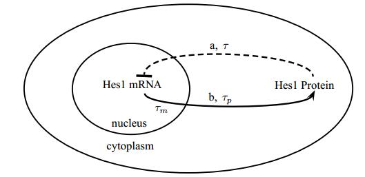
    [9] [ H. Hirata,S. Yoshiura,T. Ohtsuka,Y. Bessho,T. Harada,K. Yoshikawa,R. Kageyama, Oscillatory expression of the bhlh factor hes1 regulated by a negative feedback loop, Science, 298 (2002): 840-843.
    [10] [ Q. Hu,W. Krawcewicz,J. Turi, Global stability lobes of a state-dependent model of turning processes, SIAM J. Appl. Math., 72 (2012): 1383-1405.
    [11] [ T. Insperger,G. Stépán,J. Turi, State-dependent delay in regenerative turning processes, Nonlinear Dynamics, 47 (2007): 275-283.
    [12] [ M. Jensen,K. Sneppen,G. Tiana, Sustained oscillations and time delays in gene expression of protein hes1, FEBS Lett., null (2003): 176-177.
    [13] [ J. M. Mahaffy,C. V. Pao, Models of genetic control by repression with time delays and spatial effects, J. Math. Biol., 20 (1984): 39-57.
    [14] [ A. H. Nayfeh, Introduction to Perturbation Techniques, John Wiley & Sons, 1981.
    [15] [ R. Nussbaum, Limiting profiles for solutions of differential-delay equations, Dynamical Systems V, Lecture Notes in Mathematics, 1822 (2003): 299-342.
    [16] [ H. L. Smith, Existence and uniqueness of global solutions for a size-structured model of an insect population with variable instar duration, Rocky Mountain J. Math., 24 (1994): 311-334.
    [17] [ H. L. Smith, Oscillations and multiple steady states in a cyclic gene model with repression, J. Math. Biol., 25 (1987): 169-190.
    [18] [ P. Smolen,D. A. Baxter,J. H. Byrne, Effects of macromolecular transport and stochastic fluctuations on the dynamics of genetic regulatory systems, Am. J. Physiol., 277 (1999): C777-C790.
    [19] [ P. Smolen,D. A. Baxter,J. H. Byrne, Modeling transcriptional control in gene networks-methods, recent results, and future, Bull. Math. Biol., 62 (2000): 247-292.
    [20] [ M. Sturrock,A. J. Terry,D. P. Xirodimas,A. M. Thompson,M. A. J. Chaplain, Spatio-temporal modeling of the Hes1 and p53 Mdm2 intracellular signaling pathways, J. Theor. Biol., 273 (2011): 15-31.
    [21] [ J. Tyson,H. G. Othmer, The dynamics of feedback control circuits in biochemical pathways, Prog. Theor. Biol., 5 (1978): 2-62.
    [22] [ H.-O. Walther, Stable periodic motion of a system using echo for position control, J. Dynam. Differential Equations, 1 (2003): 143-223.
    [23] [ -, Smoothness properties of semiflows for differential equations with state-dependent delays, J. Math. Sci., 124 (2004): 5193-5207.
    [24] [ A. Wan,X. Zou, Hopf bifurcation analysis for a model of genetic regulatory system with delay, J. Math. Anal. Appl., 356 (2009): 464-476.
    [25] [ B. Wu,C. Eliscovich,Y. J. Yoon,R. H. Singer, Translation dynamics of single mRNAs in live cells and neurons, Science, 352 (2016): 1430-1435.
  • This article has been cited by:

    1. Vincenzo M. Isaia, A Fixed Point Approach to Simulation of Functional Differential Equations with a Delayed Argument, 2021, 1040-7294, 10.1007/s10884-021-10081-7
    2. Xiaodi Li, Dongxue Peng, Uniform stability of nonlinear systems with state-dependent delay, 2022, 137, 00051098, 110098, 10.1016/j.automatica.2021.110098
  • Reader Comments
  • © 2018 the Author(s), licensee AIMS Press. This is an open access article distributed under the terms of the Creative Commons Attribution License (http://creativecommons.org/licenses/by/4.0)
通讯作者: 陈斌, bchen63@163.com
  • 1. 

    沈阳化工大学材料科学与工程学院 沈阳 110142

  1. 本站搜索
  2. 百度学术搜索
  3. 万方数据库搜索
  4. CNKI搜索

Metrics

Article views(3737) PDF downloads(650) Cited by(2)

Article outline

Other Articles By Authors

/

DownLoad:  Full-Size Img  PowerPoint
Return
Return

Catalog