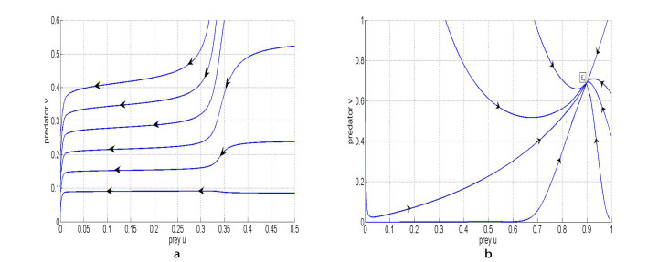
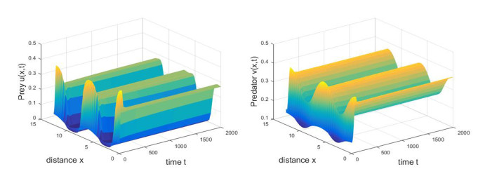
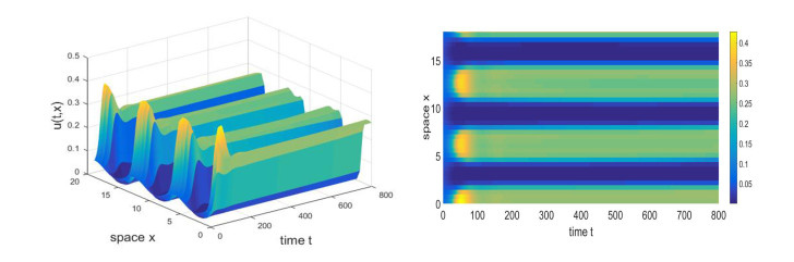
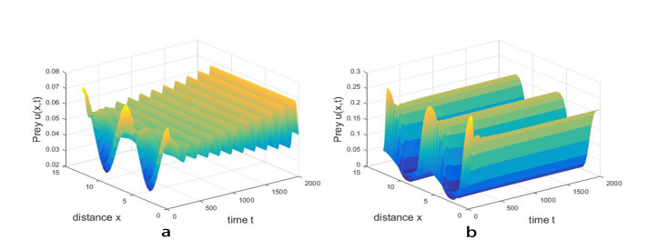
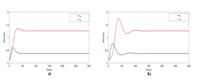
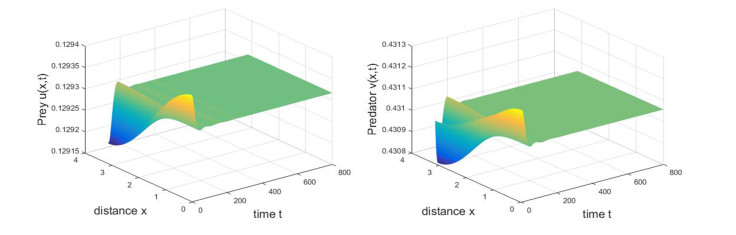
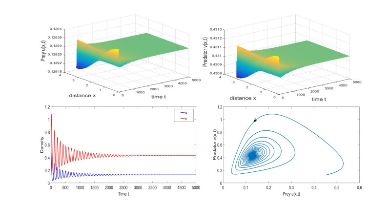
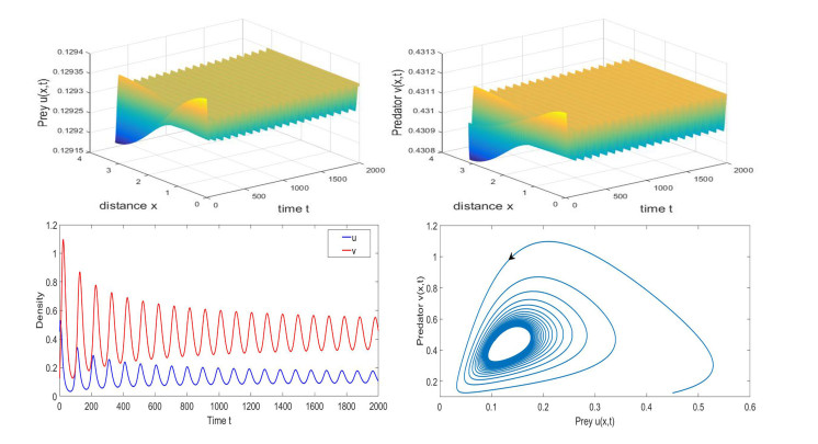
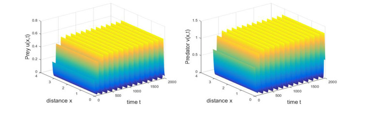
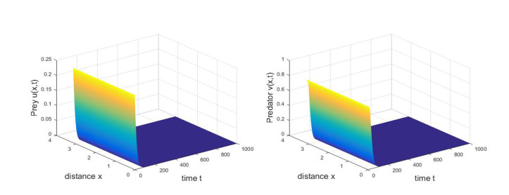
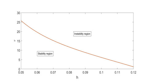
Based on ecological significance, a delayed diffusive predator-prey system with food-limited and nonlinear harvesting subject to the Neumann boundary conditions is investigated in this paper. Firstly, the sufficient conditions of the stability of nonnegative constant steady state solutions of system are derived. The existence of Hopf bifurcation is obtained by analyzing the associated characteristic equation and the conditions of Turing instability are derived when the system has no delay. Furthermore, the occurrence conditions the Hopf bifurcation are discussed by regarding delay expressing the gestation time of the predator as the bifurcation parameter. Secondly, by using upper-lower solution method, the global asymptotical stability of a unique positive constant steady state solution of system is investigated. Moreover, we also give the detailed formulas to determine the direction, stability of Hopf bifurcation by applying the normal form theory and center manifold reduction. Finally, numerical simulations are carried out to demonstrate our theoretical results.
Citation: Guangxun Sun, Binxiang Dai. Stability and bifurcation of a delayed diffusive predator-prey system with food-limited and nonlinear harvesting[J]. Mathematical Biosciences and Engineering, 2020, 17(4): 3520-3552. doi: 10.3934/mbe.2020199
Based on ecological significance, a delayed diffusive predator-prey system with food-limited and nonlinear harvesting subject to the Neumann boundary conditions is investigated in this paper. Firstly, the sufficient conditions of the stability of nonnegative constant steady state solutions of system are derived. The existence of Hopf bifurcation is obtained by analyzing the associated characteristic equation and the conditions of Turing instability are derived when the system has no delay. Furthermore, the occurrence conditions the Hopf bifurcation are discussed by regarding delay expressing the gestation time of the predator as the bifurcation parameter. Secondly, by using upper-lower solution method, the global asymptotical stability of a unique positive constant steady state solution of system is investigated. Moreover, we also give the detailed formulas to determine the direction, stability of Hopf bifurcation by applying the normal form theory and center manifold reduction. Finally, numerical simulations are carried out to demonstrate our theoretical results.

| [1] |
F. Smith, Population dynamics in Daphnia Magna and a new model for population growth, Ecology, 44 (1963), 651-663. doi: 10.2307/1933011

|
| [2] |
A. Wan, J. Wei, Hopf bifurcation analysis of a food-limited population model with delay, Nonlinear Anal. RWA, 11 (2010), 1087-1095. doi: 10.1016/j.nonrwa.2009.01.052
|
| [3] |
K. Gopalsamy, M. Kulenovic, G. Ladas, Time lags in a food-limited population model, Appl. Anal., 31 (1988), 225-237. doi: 10.1080/00036818808839826
|
| [4] |
X. Yang, Global attractivity in delayed differential equations with applications to "food-limited" population model, J. Math. Anal. Appl., 344 (2008), 1036-1047. doi: 10.1016/j.jmaa.2008.03.038
|
| [5] |
Y. Su, A. Wan, J. Wei, Bifurcation analysis in a diffusive food-limited model with time delay, Appl. Anal., 89 (2010), 1161-1181. doi: 10.1080/00036810903116010
|
| [6] |
S. Gourley, J. So, Dynamics of a food-limited population model incorporating nonlocal delays on a finite domain, J. Math. Biol., 44 (2002), 49-78. doi: 10.1007/s002850100109
|
| [7] |
K. Gopalsamy, M. Kulenovic, G. Ladas, Environmental periodicity and time delay in a foodlimited population-model, J. Math. Anal. Appl., 147 (1990), 545-555. doi: 10.1016/0022-247X(90)90369-Q
|
| [8] |
F. Chen, D. Sun, J. Shi, Periodicity in a food-limited population model with toxicants and state dependent delays, J. Math. Anal. Appl., 288 (2003), 136-146. doi: 10.1016/S0022-247X(03)00586-9
|
| [9] |
M. Fan, K. Wang, Periodicity in a food-limited population model with toxicants and time delays, Acta Math. Appl. Sin., 18 (2002), 309-314. doi: 10.1007/s102550200030
|
| [10] |
S. Tang, L. Chen, Global attractivity in a food-limited population model with impulsive effects, J. Math. Anal. Appl., 292 (2004), 211-221. doi: 10.1016/j.jmaa.2003.11.061
|
| [11] |
Z. Wang, W. Li, Monotone travelling fronts of a food-limited population model with nonlocal delay, Nonlinear Anal. RWA, 8 (2007), 699-712. doi: 10.1016/j.nonrwa.2006.03.001
|
| [12] | B. Yang, Pattern formation in a diffusive ratio-dependent Holling-Tanner predator-prey model with Smith growth, Discrete Dyn. Nat. Soc., 2013 (2013), 454209. |
| [13] | Z. Yue, W. Wang, Qualitative analysis of a diffusive ratio-dependent Holling-Tanner predator-prey model with Smith growth, Discrete Dyn. Nat. Soc., 2013 (2013), 267173. |
| [14] |
M. Li, H. Shu, Multiple stable periodic oscillations in a mathematical model of CTL-response to HTLV-Ⅰ infection, Bull. Math. Biol., 73 (2011), 1774-1793. doi: 10.1007/s11538-010-9591-7
|
| [15] |
A. Maiti, B. Dubey, J. Tushar, A delayed prey-predator model with Crowley-Martin-type functional response including prey refuge, Math. Methods Appl. Sci., 40 (2017), 5792-5809. doi: 10.1002/mma.4429
|
| [16] |
C. Pao, Systems of parabolic equations with continuous and discrete delays, J. Math. Anal. Appl., 205 (1997), 157-185. doi: 10.1006/jmaa.1996.5177
|
| [17] |
S. Ruan, On nonlinear dynamics of predator-prey models with discrete delay, Math. Mod. Nat. Phen., 4 (2009), 140-188. doi: 10.1051/mmnp/20094207
|
| [18] |
H. Shu, L. Wang, J. Watmough, Sustained and transient oscillations and chaos induced by delayed antiviral inmune response in an immunosuppressive infective model, J. Math. Biol., 68 (2014), 477-503. doi: 10.1007/s00285-012-0639-1
|
| [19] |
Y. Song, M. Han, J. Wei, Stability and Hopf bifurcation analysis on a simplified BAM neural network with delays, Phys. D, 200 (2005), 185-204. doi: 10.1016/j.physd.2004.10.010
|
| [20] |
G. Wolkowicz, H. Xia, Global asymptotic behavior of chemostat model with discrete delays, SIAM J. Appl. Math., 57 (1997), 1019-1043. doi: 10.1137/S0036139995287314
|
| [21] | D. Xiao, Dynamics and bifurcations on a class of population model with seasonal constant-yield harvesting, Discrete Contin. Dyn. Syst. B, 21 (2007), 699-719. |
| [22] |
R. Gupta, P. Chandra, Bifurcation analysis of modified Leslie-Gower predator-prey model with Michaelis-Menten type prey harvesting, J. Math. Anal. Appl., 398 (2013), 278-295. doi: 10.1016/j.jmaa.2012.08.057
|
| [23] | H. Zhao, X. Zhang, X. Huang, Hopf bifurcation and spatial patterns of a delayed biological economic system with diffusion, Appl. Math. Comput., 266 (2015), 462-480. |
| [24] |
H. Fang, Existence of eight positive periodic solutions for a food-limited two-species cooperative patch system with harvesting terms, Commun. Nonlinear Sci. Numer. Simulat., 18 (2013), 1857-1869. doi: 10.1016/j.cnsns.2012.12.002
|
| [25] |
H. Fang, Multiple positive periodic solutions for a food-limited two-species ratio-dependent predator-prey patch system with delay and harvesting, Electron. J. Differ. Equ., 2012 (2012), 1-13. doi: 10.1186/1687-1847-2012-1
|
| [26] |
X. Meng, J. Li, Stability and Hopf bifurcation analysis of a delayed phytoplankton-zooplankton model with Allee effect and linear harvesting, Math. Biosci. Eng., 17 (2020), 1973-2002. doi: 10.3934/mbe.2020105
|
| [27] |
S. Guo, S. Yan, Hopf bifurcation in a diffusion Lotka-Volterra type system with nonlocal delay effect, J. Differ. Equ., 260 (2016), 781-817. doi: 10.1016/j.jde.2015.09.031
|
| [28] | R. Han, B. Dai, Spatiotemporal dynamics and spatial pattern in a diffusive intraguild predation model with delay effect, Appl. Math. Comput., 312 (2017), 177-201. |
| [29] |
R. Han, B. Dai, Cross-diffusion induced Turing instability and amplitude equation for a toxicphytoplankton-zooplankton model with nonmonotonic functional response, Int. J. Bifurcat. Chaos, 27 (2017), 1750088. doi: 10.1142/S0218127417500882
|
| [30] |
R. Han, B. Dai, Spatiotemporal pattern formation and selection induced by nonlinear crossdiffusion in a toxic-phytoplankton-zooplankton model with Allee effect, Nonlinear Anal. RWA, 45 (2019), 822-853. doi: 10.1016/j.nonrwa.2018.05.018
|
| [31] |
D. Wu, H. Zhao, Y. Yuan, Complex dynamics of a diffusive predator-prey model with strong Allee effect and threshold harvesting, J. Math. Anal. Appl., 469 (2019), 982-1014. doi: 10.1016/j.jmaa.2018.09.047
|
| [32] |
R. Yang, J. Wei, Stability and bifurcation analysis of a diffusive prey-predator system in Holling Type Ⅲ with a prey refuge, Nonlinear Dynam., 79 (2015), 631-646. doi: 10.1007/s11071-014-1691-8
|
| [33] |
R. Yang, C. Zhang, Dynamics in a diffusive modified Leslie-Gower predator-prey model with time delay and prey harvesting, Nonlinear Dynam., 87 (2017), 863-878. doi: 10.1007/s11071-016-3084-7
|
| [34] |
H. Yin, X. Xiao, X. Wen, K. Liu, Pattern analysis of a modified Leslie-Gower predator-prey model with Crowley-Martin functional response and diffusion, Comput. Math. Appl., 67 (2014), 1607-1621. doi: 10.1016/j.camwa.2014.02.016
|
| [35] |
F. Zhang, Y. Li, Stability and Hopf bifurcation of a delayed-diffusive predator-prey model with hyperbolic mortality and nonlinear prey harvesting, Nonlinear Dynam., 88 (2017), 1397-1412. doi: 10.1007/s11071-016-3318-8
|
| [36] | Q. Ye, Z. Li, M. Wang, Y. Wu, Introduction to Reaction-diffusion Equations (2nd edition), Science Press, Beijing, 2011. |
| [37] | D. Murray, Mathematical biology Ⅱ, in Spatial Models and Biomedical Applications, SpringerVerlag, 2003. |
| [38] |
A. Turing, The chemical basis of mokmorphogenesis, Philo. Trans. Roy. Soc. London Ser. B, 237 (1952), 37-72. doi: 10.1098/rstb.1952.0012
|
| [39] |
M. Wang, P.Y. Pang, Global asymptotic stability of positive steady states of a diffusive ratiodependent prey-predator model, Appl. Math. Lett., 21 (2008), 1215-1220. doi: 10.1016/j.aml.2007.10.026
|
| [40] | J. Wu, Theory and Applications of Partial Functional Differential Equations, Springer-Verlag, New York, 1996. |
| [41] | B. Hassard, N. Kazarinoff, Y. Wan, Theory and Applications of Hopf Bifurcation, Cambridge University Press, Cambridge, 1981. |
| [42] |
Y. Song, S. Wu, H. Wang, Spatiotemporal dynamics in the single population model with memorybased diffusion and nonlocal effect, J. Differ. Equ., 267 (2019), 6316-6351. doi: 10.1016/j.jde.2019.06.025
|
Figures(11)

Guangxun Sun, Binxiang Dai. Stability and bifurcation of a delayed diffusive predator-prey system with food-limited and nonlinear harvesting[J]. Mathematical Biosciences and Engineering, 2020, 17(4): 3520-3552. doi: 10.3934/mbe.2020199


 DownLoad: