A novel fixed-point based two-step inertial algorithm for convex minimization in deep learning data classification

Kobkoon Janngam; Suthep Suantai; Rattanakorn Wattanataweekul; Kobkoon Janngam; Suthep Suantai; Rattanakorn Wattanataweekul

doi:10.3934/math.2025283

AIMS Mathematics

2025, Volume 10, Issue 3: 6209-6232. doi: 10.3934/math.2025283

Previous Article Next Article

Research article Special Issues

A novel fixed-point based two-step inertial algorithm for convex minimization in deep learning data classification

1.
Department of Mathematics, Faculty of Science, Chiang Mai University, Chiang Mai 50200, Thailand
2.
Office of Research Administration, Chiang Mai University, Chiang Mai 50200, Thailand
3.
Research Center in Optimization and Computational Intelligence for Big Data Prediction, Department of Mathematics, Faculty of Science, Chiang Mai University, Chiang Mai 50200, Thailand
4.
Department of Mathematics, Statistics and Computer, Faculty of Science, Ubon Ratchathani University, Ubon Ratchathani 34190, Thailand

Received: 30 December 2024 Revised: 22 February 2025 Accepted: 10 March 2025 Published: 19 March 2025
MSC : 47H09, 65K10, 68T07, 90C25, 90C30

In this paper, we present a novel two-step inertial algorithm for finding a common fixed-point of a countable family of nonexpansive mappings. Under mild assumptions, we prove a weak convergence theorem for the method. We then demonstrate its versatility by applying it to convex minimization problems and extending it to data classification tasks, specifically through a multihidden-layer extreme learning machine (MELM). Numerical experiments show that our approach outperforms existing methods in both convergence speed and classification accuracy. These results highlight the potential of the proposed algorithm for broader applications in machine learning and optimization.
- convex minimization problem,
- data classification,
- deep learning,
- fixed-point,
- optimization,
- two-step inertial algorithm
Citation: Kobkoon Janngam, Suthep Suantai, Rattanakorn Wattanataweekul. A novel fixed-point based two-step inertial algorithm for convex minimization in deep learning data classification[J]. AIMS Mathematics, 2025, 10(3): 6209-6232. doi: 10.3934/math.2025283

Related Papers:

Abstract

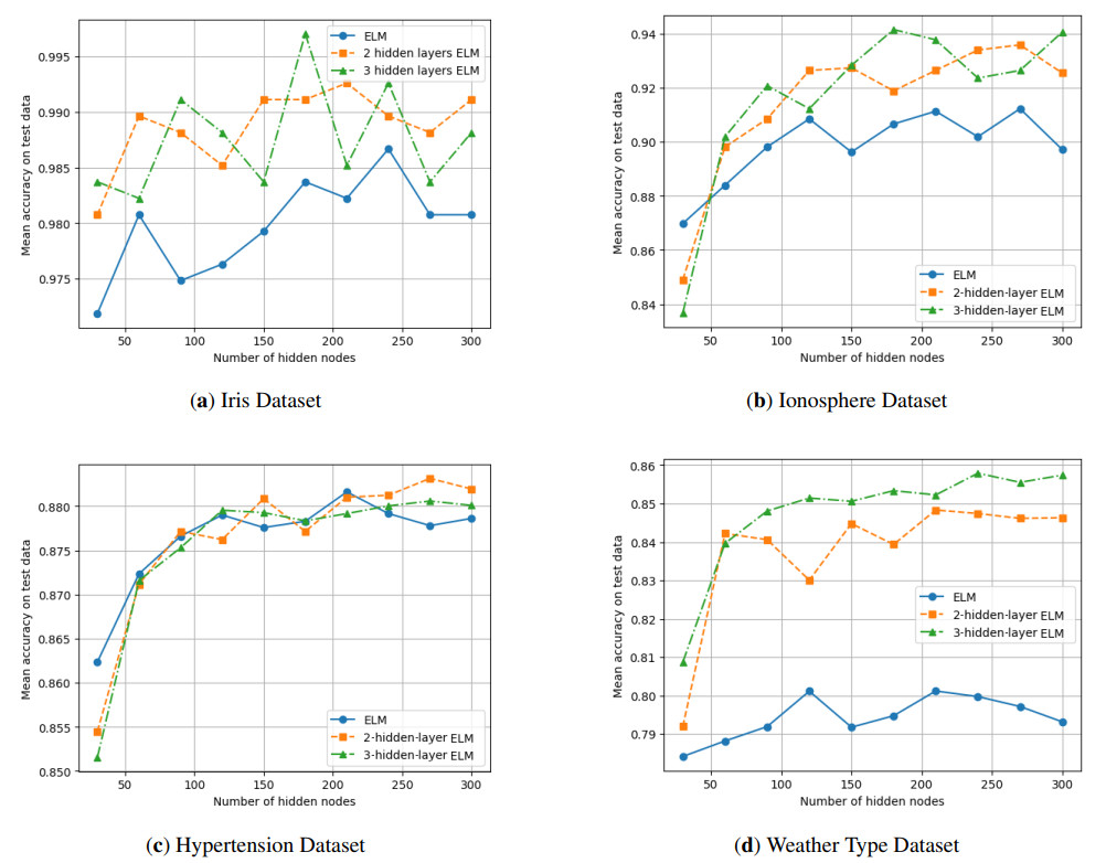
In this paper, we present a novel two-step inertial algorithm for finding a common fixed-point of a countable family of nonexpansive mappings. Under mild assumptions, we prove a weak convergence theorem for the method. We then demonstrate its versatility by applying it to convex minimization problems and extending it to data classification tasks, specifically through a multihidden-layer extreme learning machine (MELM). Numerical experiments show that our approach outperforms existing methods in both convergence speed and classification accuracy. These results highlight the potential of the proposed algorithm for broader applications in machine learning and optimization.

References

[1]	S. Boyd, L. Vandenberghe, Convex optimization, Cambridge University Press, 2004.
[2]	C. M. Bishop, Pattern recognition and machine learning, New York: Springer, 2006.
[3]	P. L. Combettes, J. C. Pesquet, Proximal splitting methods in signal processing, In: Fixed-point algorithms for inverse problems in science and engineering, New York: Springer, 2011. https://doi.org/10.1007/978-1-4419-9569-8_10
[4]	H. Markowitz, Portfolio selection, J. Financ., 7 (1952), 77–91. https://doi.org/10.1111/j.1540-6261.1952.tb01525.x
[5]	Y. Nesterov, Introductory lectures on convex optimization: A basic course, New York: Springer, 2013. https://doi.org/10.1007/978-1-4419-8853-9
[6]	R. E. Bruck Jr., On the weak convergence of an ergodic iteration for the solution of variational inequalities for monotone operators in Hilbert space, J. Math. Anal. Appl., 61 (1977), 159–164. https://doi.org/10.1016/0022-247X(77)90152-4 doi: 10.1016/0022-247X(77)90152-4
[7]	P. L. Lions, B. Mercier, Splitting algorithms for the sum of two nonlinear operators, SIAM J. Numer. Anal., 16 (1979), 964–979. https://doi.org/10.1137/0716071 doi: 10.1137/0716071
[8]	A. Cabot, Proximal point algorithm controlled by a slowly vanishing term: applications to hierarchical minimization, SIAM J. Optim., 15 (2005), 555–572. https://doi.org/10.1137/S105262340343467X doi: 10.1137/S105262340343467X
[9]	H. K. Xu, Averaged mappings and the gradient-projection algorithm, J. Optim. Theory Appl., 150 (2011), 360–378. https://doi.org/10.1007/s10957-011-9837-z doi: 10.1007/s10957-011-9837-z
[10]	J. J. Moreau, Fonctions convexes duales et points proximaux dans un espace hilbertien, C. R. Acad. Sci. Paris Ser. A Math., 255 (1962), 2897–2899.
[11]	P. L. Combettes, V. R. Wajs, Signal recovery by proximal forward-backward splitting, Multiscale Model. Sim., 4 (2005), 1168–1200. https://doi.org/10.1137/050626090 doi: 10.1137/050626090
[12]	L. Bussaban, S. Suantai, A. Kaewkhao, A parallel inertial S-iteration forward-backward algorithm for regression and classification problems, Carpathian J. Math., 36 (2020), 35–44. https://doi.org/10.37193/CJM.2020.01.04 doi: 10.37193/CJM.2020.01.04
[13]	M. Bačák, S. Reich, The asymptotic behavior of a class of nonlinear semigroups in Hadamard spaces, J. Fixed Point Theory Appl., 16 (2014), 189–202. https://doi.org/10.1007/s11784-014-0202-3 doi: 10.1007/s11784-014-0202-3
[14]	K. Janngam, S. Suantai, Y. J. Cho, A. Kaewkhao, R. Wattanataweekul, A novel inertial viscosity algorithm for bilevel optimization problems applied to classification problems, Mathematics, 11 (2023), 3241. https://doi.org/10.3390/math11143241 doi: 10.3390/math11143241
[15]	R. Wattanataweekul, K. Janngam, S. Suantai, A novel two-step inertial viscosity algorithm for bilevel optimization problems applied to image recovery, Mathematics, 11 (2023), 3518. https://doi.org/10.3390/math11163518 doi: 10.3390/math11163518
[16]	A. Beck, M. Teboulle, A fast iterative shrinkage-thresholding algorithm for linear inverse problems, SIAM J. Imaging Sci., 2 (2009), 183–202. https://doi.org/10.1137/080716542 doi: 10.1137/080716542
[17]	Y. Nesterov, A method of solving a convex programming problem with convergence rate $O(1/k^2)$, Dokl. Akad. Nauk SSSR, 269 (1983), 543–547.
[18]	A. Kaewkhao, L. Bussaban, S. Suantai, Convergence theorem of inertial P-iteration method for a family of nonexpansive mappings with applications, Thai J. Math., 18 (2020), 1743–1751.
[19]	P. Thongsri, S. Suantai, New accelerated fixed-point algorithms with applications to regression and classification problems, Thai J. Math., 18 (2020), 2001–2011.
[20]	K. Janngam, S. Suantai, An accelerated forward-backward algorithm with applications to image restoration problems, Thai J. Math., 19 (2021), 325–339.
[21]	P. Sae-jia, S. Suantai, A novel algorithm for convex bi-level optimization problems in Hilbert spaces with applications, Thai J. Math., 21 (2023), 625–645.
[22]	D. Reem, S. Reich, A. De Pierro, A telescopic Bregmanian proximal gradient method without the global Lipschitz continuity assumption, J. Optim. Theory Appl., 182 (2019), 851–884. https://doi.org/10.48550/arXiv.1804.10273 doi: 10.48550/arXiv.1804.10273
[23]	C. Izuchukwu, M. Aphane, K. O. Aremu, Two-step inertial forward-reflected-anchored-backward splitting algorithm for solving monotone inclusion problems, Comp. Appl. Math., 42 (2023), 351. https://doi.org/10.1007/s40314-023-02485-6 doi: 10.1007/s40314-023-02485-6
[24]	O. S. Iyiola, Y. Shehu, Convergence results of two-step inertial proximal point algorithm, Appl. Numer. Math., 182 (2022), 57–75. https://doi.org/10.1016/j.apnum.2022.07.013 doi: 10.1016/j.apnum.2022.07.013
[25]	D. V. Thong, S. Reich, X. H. Li, P. T. H. Tham, An efficient algorithm with double inertial steps for solving split common fixed-point problems and an application to signal processing, Comp. Appl. Math., 44 (2025), 102 https://doi.org/10.1007/s40314-024-03058-x doi: 10.1007/s40314-024-03058-x
[26]	K. Nakajo, K. Shimoji, W. Takahashi, Strong convergence to a common fixed-point of families of nonexpansive mappings in Banach spaces, J. Nonlinear Convex A., 8 (2007), 11.
[27]	H. H. Bauschke, P. L. Combettes, Convex analysis and monotone operator theory in Hilbert spaces, Cham: Springer, 2017. https://doi.org/10.1007/978-3-319-48311-5
[28]	R. E. Bruck, S. Reich, Nonexpansive projections and resolvents of accretive operators in Banach spaces, Houston J. Math., 3 (1977), 459–470.
[29]	K. Tan, H. K. Xu, Approximating fixed-points of nonexpansive mappings by the Ishikawa iteration process, J. Math. Anal. Appl., 178 (1993), 301–308. https://doi.org/10.1006/jmaa.1993.1309 doi: 10.1006/jmaa.1993.1309
[30]	W. Takahashi, Introduction to nonlinear and convex analysis, Yokohama Publishers, 2009.
[31]	A. Moudafi, E. Al-Shemas, Simultaneous iterative methods for split equality problem, Trans. Math. Program. Appl., 1 (2013), 1–11.
[32]	Y. LeCun, Y. Bengio, G. Hinton, Deep learning, Nature, 521 (2015), 436–444. https://doi.org/10.1038/nature14539 doi: 10.1038/nature14539
[33]	J. Schmidhuber, Deep learning in neural networks: An overview, Neural Netw., 61 (2015), 85–117. https://doi.org/10.1016/j.neunet.2014.09.003 doi: 10.1016/j.neunet.2014.09.003
[34]	D. E. Rumelhart, G. E. Hinton, R. J. Williams, Learning representations by back-propagating errors, Nature, 323 (1986), 533–536. https://doi.org/10.1038/323533a0 doi: 10.1038/323533a0
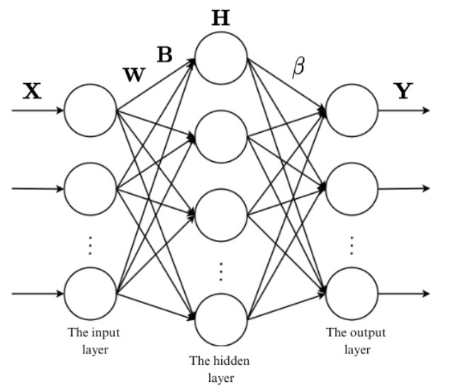
[35]	G. B. Huang, Q. Y. Zhu, C. K. Siew, Extreme learning machine: Theory and applications, Neurocomputing, 70 (2006), 489–501. https://doi.org/10.1016/j.neucom.2005.12.126 doi: 10.1016/j.neucom.2005.12.126
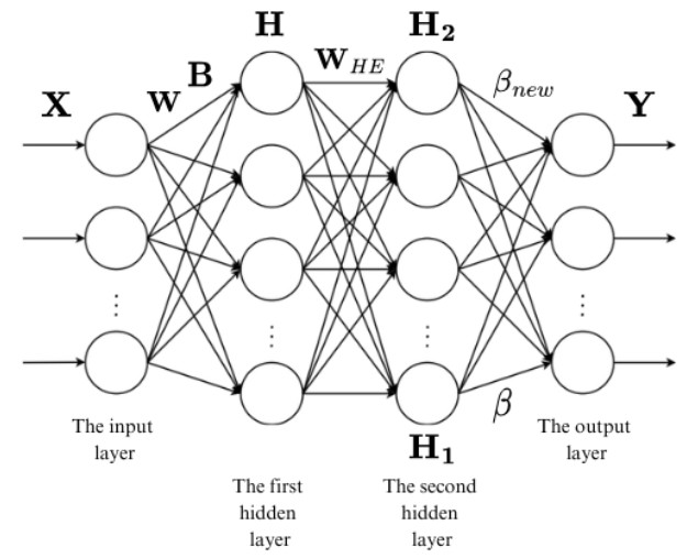
[36]	B. Y. Qu, B. F. Lang, J. J. Liang, A. K. Qin, O. D. Crisalle, Two-hidden-layer extreme learning machine for regression and classification, Neurocomputing, 175 (2016), 826–834. https://doi.org/10.1016/j.neucom.2015.11.009 doi: 10.1016/j.neucom.2015.11.009
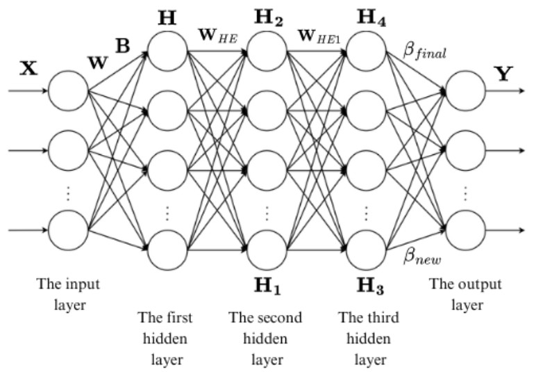
[37]	D. Xiao, B. Li, Y. Mao, A multiple hidden layers extreme learning machine method and its application, Math. Probl. Eng., 2017 (2017), 4670187. https://doi.org/10.1155/2017/4670187 doi: 10.1155/2017/4670187
[38]	R. Tibshirani, Regression shrinkage and selection via the lasso, J. R. Stat. Soc. B, 58 (1996), 267–288. https://doi.org/10.1111/j.2517-6161.1996.tb02080.x doi: 10.1111/j.2517-6161.1996.tb02080.x
[39]	R. A. Fisher, Iris, UCI machine learning repository, 1988. https://doi.org/10.24432/C56C76
[40]	V. Sigillito, S. Wing, L. Hutton, K. Baker, Ionosphere, UCI machine learning repository, 1989.
[41]	Nikhil7280, Weather type classification dataset, Kaggle, 2021. Available from: https://www.kaggle.com/datasets/nikhil7280/weather-type-classification/data.

Reader Comments

Your name:*

Email:*
© 2025 the Author(s), licensee AIMS Press. This is an open access article distributed under the terms of the Creative Commons Attribution License (http://creativecommons.org/licenses/by/4.0)