A new flexible Weibull distribution for modeling real-life data: Improved estimators, properties, and applications

Ahmed Z. Afify; Rehab Alsultan; Abdulaziz S. Alghamdi; Hisham A. Mahran; Ahmed Z. Afify; Rehab Alsultan; Abdulaziz S. Alghamdi; Hisham A. Mahran

doi:10.3934/math.2025270

AIMS Mathematics

2025, Volume 10, Issue 3: 5880-5927. doi: 10.3934/math.2025270

Previous Article Next Article

Research article

A new flexible Weibull distribution for modeling real-life data: Improved estimators, properties, and applications

1.
Department of Statistics, Mathematics, and Insurance, Benha University, Benha 13511, Egypt
2.
Mathematics Department, Faculty of Sciences, Umm AL-Qura University, Makkah 24382, Saudi Arabia
3.
Department of Mathematics, College of Science & Arts, King Abdulaziz University, P.O. Box 344, Rabigh 21911, Saudi Arabia
4.
Department of Statistics, Mathematics, and Insurance, Ain Shams University, Cairo 11566, Egypt

Received: 09 December 2024 Revised: 28 January 2025 Accepted: 13 February 2025 Published: 18 March 2025
MSC : 60E05, 62F10, 62N05

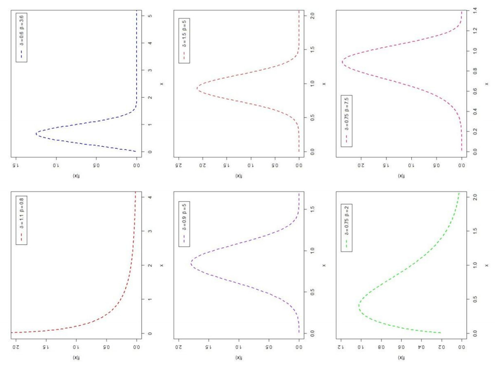
In this paper, we proposed a novel and flexible lifetime model, the generalized Kavya–Manoharan Weibull distribution, which can be interpreted as a proportional reversed hazard model. The most remarkable feature of the proposed model is its ability to effectively capture a wide range of hazard rate patterns using only three parameters. These include decreasing, J-shaped, reverse J-shaped, and increasing patterns, as well as key nonmonotonic shapes such as the bathtub, modified bathtub, and upside-down bathtub shapes. Additionally, its density can exhibit right-skewness, left-skewness, symmetry, and reversed-J shapes. We explored several distributional properties of the proposed model and estimated its parameters using eight methods. The effectiveness of these estimators was validated through extensive simulation studies. Furthermore, we assessed the versatility of the proposed distribution using three real-world datasets, demonstrating its exceptional capacity to fit the data accurately. Our results indicated that the proposed distribution outperforms several existing generalizations of the Weibull distribution in terms of fit quality.
- GKM-G family,
- Weibull distribution,
- quantile function,
- order statistics,
- parameter estimation,
- failure time data
Citation: Ahmed Z. Afify, Rehab Alsultan, Abdulaziz S. Alghamdi, Hisham A. Mahran. A new flexible Weibull distribution for modeling real-life data: Improved estimators, properties, and applications[J]. AIMS Mathematics, 2025, 10(3): 5880-5927. doi: 10.3934/math.2025270

Related Papers:

Abstract

In this paper, we proposed a novel and flexible lifetime model, the generalized Kavya–Manoharan Weibull distribution, which can be interpreted as a proportional reversed hazard model. The most remarkable feature of the proposed model is its ability to effectively capture a wide range of hazard rate patterns using only three parameters. These include decreasing, J-shaped, reverse J-shaped, and increasing patterns, as well as key nonmonotonic shapes such as the bathtub, modified bathtub, and upside-down bathtub shapes. Additionally, its density can exhibit right-skewness, left-skewness, symmetry, and reversed-J shapes. We explored several distributional properties of the proposed model and estimated its parameters using eight methods. The effectiveness of these estimators was validated through extensive simulation studies. Furthermore, we assessed the versatility of the proposed distribution using three real-world datasets, demonstrating its exceptional capacity to fit the data accurately. Our results indicated that the proposed distribution outperforms several existing generalizations of the Weibull distribution in terms of fit quality.

References

[1]	C. Lee, F. Famoye, O. Olumolade, Beta-Weibull distribution: some properties and applications to censored data, J. Mod. Appl. Stat. Meth., 6 (2007), 173–186.
[2]	G. M. Cordeiro, E. M. M. Ortega, S. Nadarajah, The Kumaraswamy Weibull distribution with application to failure data, J. Franklin I., 347 (2010), 1399–1429.https://doi.org/10.1016/j.jfranklin.2010.06.010 doi: 10.1016/j.jfranklin.2010.06.010
[3]	T. Zhang, M. Xie, On the upper truncated Weibull distribution and its reliability implications, Reliab. Eng. Syst. Safe., 96 (2011), 194–200.https://doi.org/10.1016/j.ress.2010.09.004 doi: 10.1016/j.ress.2010.09.004
[4]	G. R. Aryal, C. P. Tsokos, Transmuted Weibull distribution: a generalization of the Weibull probability distribution, Eur. J. Pure Appl. Math., 4 (2011), 89–102.
[5]	G. M. Cordeiro, E. M. M. Ortega, D. C. C. da Cunha, The exponentiated generalized class of distributions, Journal of Data Science, 11 (2013), 1–27.https://doi.org/10.6339/JDS.2013.11(1).1086 doi: 10.6339/JDS.2013.11(1).1086
[6]	X. Peng, Z. Yan, Estimation and application for a new extended Weibull distribution, Reliab. Eng. Syst. Safe., 121 (2014), 34–42.https://doi.org/10.1016/j.ress.2013.07.007 doi: 10.1016/j.ress.2013.07.007
[7]	M. N. Khan, The modified beta Weibull distribution, Hacet. J. Math. Stat., 44 (2015), 1553–1568.
[8]	A. Z. Afify, G. M. Cordeiro, N. S. Butt, E. M. M. Ortega, A. K. Suzuki, A new lifetime model with variable shapes for the hazard rate, Braz. J. Probab. Stat., 31 (2017), 516–541.https://doi.org/10.1214/16-BJPS322 doi: 10.1214/16-BJPS322
[9]	T. H. M. Abouelmagd, S. Al-mualim, M. Elgarhy, A. Z. Afify, M. Ahmad, Properties of the four-parameter Weibull distribution and its applications, Pak. J. Statist., 33 (2017), 449–466.
[10]	M. Nassar, A. Alzaatreh, M. Mead, O. Abo-Kasem, Alpha power Weibull distribution: properties and applications, Commun. Stat. -Theory M., 46 (2017), 10236–10252.https://doi.org/10.1080/03610926.2016.1231816 doi: 10.1080/03610926.2016.1231816
[11]	A. Z. Afify, M. Alizadeh, M. Zayed, T. G. Ramires, F. Louzada, The odd log-logistic exponentiated Weibull distribution: regression modeling, properties, and applications, Iran. J. Sci. Technol. Trans. Sci., 42 (2018). 2273–2288.https://doi.org/10.1007/s40995-018-0524-x doi: 10.1007/s40995-018-0524-x
[12]	G. M. Cordeiro, A. Z. Afify, H. M. Yousof, S. Cakmakyapan, G. Ozel, The Lindley Weibull distribution: properties and applications, An. Acad. Bras. Ciênc., 90 (2018), 2579–2598.https://doi.org/10.1590/0001-3765201820170635 doi: 10.1590/0001-3765201820170635
[13]	G. S. Mudholkar, D. K. Srivastava, Exponentiated Weibull family for analyzing bathtub failure-rate data, IEEE Trans. Reliab., 42 (1993), 299–302.https://doi.org/10.1109/24.229504 doi: 10.1109/24.229504
[14]	M. Nassar, A. Z. Afify, S. Dey, D. Kumar, A new extension of Weibull distribution: properties and different methods of estimation, J. Comput. Appl. Math., 336 (2018), 439–457.https://doi.org/10.1016/j.cam.2017.12.001 doi: 10.1016/j.cam.2017.12.001
[15]	M. E. Mead, G. M. Cordeiro, A. Z. Afify, H. Al Mofleh, The alpha power transformation family: properties and applications, Pak. J. Stat. Oper. Res., 15 (2019), 525–545.https://doi.org/10.18187/pjsor.v15i3.2969 doi: 10.18187/pjsor.v15i3.2969
[16]	G. M. Cordeiro, A. Z. Afify, E. M. Ortega, A. K. Suzuki, M. E. Mead, The odd Lomax generator of distributions: properties, estimation and applications, J. Comput. Appl. Math., 347 (2019), 222–237.https://doi.org/10.1016/j.cam.2018.08.008 doi: 10.1016/j.cam.2018.08.008
[17]	A. I. Ishaq, A. A. Abiodun, The Maxwell–Weibull distribution in modeling lifetime datasets, Ann. Data Sci., 7 (2020), 639–662.https://doi.org/10.1007/s40745-020-00288-8 doi: 10.1007/s40745-020-00288-8
[18]	A. EL-Baset A. Ahmad, M. G. M. Ghazal, Exponentiated additive Weibull distribution, Reliab. Eng. Syst. Safe., 193 (2020), 106663.https://doi.org/10.1016/j.ress.2019.106663 doi: 10.1016/j.ress.2019.106663
[19]	M. Alizadeh, M. N. Khan, M. Rasekhi, G. G. Hamedani, A new generalized modified Weibull distribution, Statistics, Optimization & Information Computing, 9 (2021), 17–34.https://doi.org/10.19139/soic-2310-5070-1014 doi: 10.19139/soic-2310-5070-1014
[20]	H. M. Alshanbari, O. H. Odhah, H. Al-Mofleh, Z. Ahmad, S. K. Khosa, A. A. A. H. El-Bagoury, A new flexible Weibull extension model: different estimation methods and modeling an extreme value data, Heliyon, 9 (2023), e21704. https://doi.org/10.1016/j.heliyon.2023.e21704 doi: 10.1016/j.heliyon.2023.e21704
[21]	M. K. Refaie, A. A. Yaqoob, M. A. Selim, E. I. A. Ali, A novel version of the exponentiated Weibull distribution: copulas, mathematical properties and statistical modeling, Pak. J. Stat. Oper. Res., 19 (2023), 491–519. https://doi.org/10.18187/pjsor.v19i3.4089 doi: 10.18187/pjsor.v19i3.4089
[22]	M. M. Al Sobhi, The extended Weibull distribution with its properties, estimation and modeling skewed data, J. King Saud Univ. Sci., 34 (2022), 101801.https://doi.org/10.1016/j.jksus.2021.101801 doi: 10.1016/j.jksus.2021.101801
[23]	H. S. Klakattawi, Survival analysis of cancer patients using a new extended Weibull distribution, PLoS ONE, 17 (2022), e0264229.https://doi.org/10.1371/journal.pone.0264229 doi: 10.1371/journal.pone.0264229
[24]	P. Kumar, L. P. Sapkota, V. Kumar, N. Bam, Exploring the new exponentiated inverse weibull distribution: properties, estimation, and analysis via classical and Bayesian approaches, Contemp. Math., 6 (2025), 827–849.https://doi.org/10.37256/cm.6120256255 doi: 10.37256/cm.6120256255
[25]	T. N. Sindhu, A. Shafiq, S. A. Lone, Q. M. Al-Mdallal, T. A. Abushal, Distributional properties of the entropy transformed Weibull distribution and applications to various scientific fields, Sci. Rep., 14 (2024), 31827.https://doi.org/10.1038/s41598-024-83132-w doi: 10.1038/s41598-024-83132-w
[26]	H. M. Alshanbari, Z. Ahmad, A. H. El-Bagoury, O. H. Odhah, G. S. Rao, A new modification of the Weibull distribution: model, theory, and analyzing engineering data sets, Symmetry, 16 (2024), 611.https://doi.org/10.3390/sym16050611 doi: 10.3390/sym16050611
[27]	A. A. Suleiman, H. Daud, A. I. Ishaq, M. Kayid, R. Sokkalingam, Y. Hamed, et al., A new Weibull distribution for modeling complex biomedical data, J. Radiat. Res. Appl. Sci., 17 (2024), 101190.https://doi.org/10.1016/j.jrras.2024.101190 doi: 10.1016/j.jrras.2024.101190
[28]	H. Mahran, M. M. Mansour, E. M. Abd Elrazik, A. Z. Afify, A new one-parameter flexible family with variable failure rate shapes: properties, inference, and real-life applications, AIMS Math., 9 (2024), 11910–11940.https://doi.org/10.3934/math.2024582 doi: 10.3934/math.2024582
[29]	P. G. Sankaran, V. L. Gleeja, Proportional reversed hazard and frailty models, Metrika, 68 (2008), 333–342.https://doi.org/10.1007/s00184-007-0165-0 doi: 10.1007/s00184-007-0165-0
[30]	P. G. Sankaran, V. L. Gleeja, On proportional reversed hazards frailty models, Metron, 69 (2011), 151–173.https://doi.org/10.1007/BF03263554 doi: 10.1007/BF03263554
[31]	A. Di Crescenzo, Some results on the proportional reversed hazards model, Stat. Probabil. Lett., 50 (2000), 313–321.https://doi.org/10.1016/S0167-7152(00)00127-9 doi: 10.1016/S0167-7152(00)00127-9
[32]	R. C. Gupta, R. D. Gupta, Proportional reversed hazard rate model and its applications, J. Stat. Plan. Infer., 137 (2007), 3525–3536.https://doi.org/10.1016/j.jspi.2007.03.029 doi: 10.1016/j.jspi.2007.03.029
[33]	E. L. Lehmann, The power of rank tests, Ann. Math. Stat., 24 (1953), 23–43.
[34]	J. A. Greenwood, J. M. Landwehr, N. C. Matalas, J. R. Wallis, Probability weighted moments: definition and relation to parameters of several distributions expressible in inverse form, Water Resour. Res., 15 (1979), 1049–1054.https://doi.org/10.1029/WR015i005p01049 doi: 10.1029/WR015i005p01049
[35]	J. J. Swain, S. Venkatraman, J. R. Wilson, Least squares estimation of distribution function in Johnson's translation system, J. Stat. Comput. Sim., 29 (1988), 271–297.https://doi.org/10.1080/00949658808811068 doi: 10.1080/00949658808811068
[36]	H. Cramér, On the composition of elementary errors, Scand. Actuar. J., 1928 (1928), 13–74.https://doi.org/10.1080/03461238.1928.10416862 doi: 10.1080/03461238.1928.10416862
[37]	R. E. Von Mises, Wahrscheinlichkeit statistik und wahrheit, Basel: Springer, 1928.
[38]	R. C. H. Cheng, N. A. K. Amin, Maximum product of spacings estimation with application to the lognormal distribution, Cardiff: University of Wales Institute of Science and Technology, 1979, Math Report 79-1.
[39]	R. C. H. Cheng, N. A. K. Amin, Estimating parameters in continuous univariate distributions with a shifted origin, J. R. Stat. Soc. B, 45 (1983), 394–403.https://doi.org/10.1111/j.2517-6161.1983.tb01268.x doi: 10.1111/j.2517-6161.1983.tb01268.x
[40]	J. H. K. Kao, Computer methods for estimating Weibull parameters in reliability studies, IRE Transactions on Reliability and Quality Control, 13 (1958), 15–22.https://doi.org/10.1109/IRE-PGRQC.1958.5007164 doi: 10.1109/IRE-PGRQC.1958.5007164
[41]	D. Kundu, M. Z. Raqab, Estimation of R = P (Y < X) for three-parameter Weibull distribution, Stat. Probabil. Lett., 79 (2009), 1839–1846.https://doi.org/10.1016/j.spl.2009.05.026 doi: 10.1016/j.spl.2009.05.026
[42]	D. N. P. Murthy, M. Xie, R. Jiang, Weibull models, Hoboken: Wiley, 2004.https://doi.org/10.1002/047147326X
[43]	G. P. Patil, C. R. Rao, Volume 12: Environmental statistics, Handbook of statistics, Elsevier, 1994.

Reader Comments

Your name:*

Email:*
© 2025 the Author(s), licensee AIMS Press. This is an open access article distributed under the terms of the Creative Commons Attribution License (http://creativecommons.org/licenses/by/4.0)