Construction of a cryptographic function based on Bose-type Sidon sets

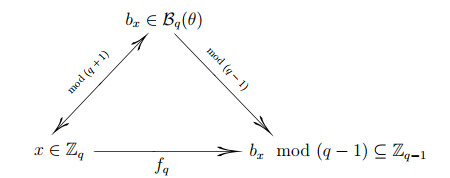
1.   Introduction

In population ecology, understanding how predators and primary producers influence nutrient flow relative to each other is important. Ecosystem interactions and predator-prey relationships are governed by predation and the delivery of resource processes. The identification of ecological factors that can alter or control dynamic behavior requires theoretical and experimental research. One way to study these questions is by means of experimental control, and another useful way is via mathematical modeling as well as computer simulations. Over decades of theoretical ecology and biomathematics development, mathematical modeling has become an indispensable tool for scientists in related fields to study ecosystems. Since Lotka [1] and Volterra [2], as cornerstones of theoretical ecology, published the first study of predator-prey dynamics, any species in nature can be a predator or prey, and due to its prevalence, it has become one of the most popular topics for researchers to study [3,4,5]. Besides, because biological resources are renewable and have the most unique development mechanisms, the over-utilization of biological resources and the destruction of the environment by humans will directly affect the balance of the ecosystem. Maintaining ecological balance and meeting humans material needs have attracted the most attention from researchers focused on the scientific management of renewable resource development [6,7,8].

Shelter serves as a defense strategy. It refers broadly to a series of behaviors by prey to avoid predators in order to increase their survival rate. The concept of sanctuary was first developed by Maynard-Smith [9] and Gause et al. [10], and its popularity has been very high, garnering widespread attention from many scholars [11,12,13,14,15]. Sih et al.[16] investigated the effects of prey refuge in a three-species model and concluded that the system's stability is strongly related to the refuge. Also, similar findings can be displayed in [17,18,19,20,21,22]. The two modes of refuge analyzed by Gonzalez-Olivares et al. [17] have diverse stability domains in terms of the parameter space. Qi et al.[21] ensure the stability of the system by varying the strength of the refuge.

Through reviewing a large amount of literature, we begin to consider [23,24] as a basis for the two prey and one predator species that will be modeled in this article. We assume that at a certain time $t$, the populations of the two prey and one predator are $x_1(t)$, $x_2(t)$, and $y(t)$, respectively. Based on the above, we construct the following model:

The significance of the full parameters is annotated in Table 1.

Most species in nature, including humans, are influenced by fear. Fear may cause an abnormal state and behavior to arise. As usual, prey have an innate fear of predators. The ecology of fear is related to combining the optimal behavior of prey and predators with their population densities [25,26]. In view of reality, it is a fact that prey fear predators, which is seen as a psychological effect that can have a lasting impact on prey populations. This psychological influence is often easy to overlook, but it is necessary to consider it in the context of practical ecology [27]. Wang et al. [28] first considered the effect of the fear factor on the model and first proposed the fear of prey $F(k, y)$. Afterwards, some researchers have investigated the effects of the fear effect and predator interferences in some three-dimensional systems as well as explored the generation of Hopf bifurcation conditions in the presence of a fear parameter as a bifurcation parameter [29,30,31,32]. Zanette et al. [33] observed that prey will reduce reproducing because of fear of being killed by predators, thus decreasing the risk of being killed after giving birth, which also leads directly to a decline in prey birth rates. According to the above discussion, our paper considers the different fears $k_i$ caused by predators for the two prey species.

In reality, when prey feel the crisis of being hunted, they will reproduce less and increase their survival rate. These conditions about the fear factor $F(k_i, y)$ $(i = 1, 2)$ are listed as follows:

$\mathbf{1})$ $F(0, y) = 1$: prey production does not decrease when the prey does not fear the predator;

$\mathbf{2})$ $F(k_i, 0) = 1$: even though the prey will develop a fear of predators and there will be no predators, prey production will still not decline;

$\mathbf{3})$ $\lim\limits_{k_i\rightarrow \infty} F(k_i, y) = 0$: when the prey's fear of the predator is very high, this will result in the prey production tending to zero;

$\mathbf{4})$ $\lim\limits_{y\rightarrow \infty} F(k_i, y) = 0$: prey have a fear of predators, and when predator numbers are too large, this can also lead to prey production tending to zero;

$\mathbf{5})$ $\frac{\partial F(k_i, y)}{\partial k_i} < 0$: the greater the prey's fear of predators, the less productive it will be;

$\mathbf{6})$ $\frac{\partial F(k_i, y)}{\partial y} < 0$: predators are inversely proportional to their prey.

For ease of analysis, we draw on Wang et al. [28] to consider the fear effect:

obviously, $F(k_i, y)$ $(i = 1, 2)$ in (1.2) satisfies conditions $\mathbf{1})$–$\mathbf{6})$. Based on the above conditions, this study will consider the effect of fear on system (1.1) to obtain system (1.3).

Notably, most biological parameters in much of the literature are fixed constants. However, in reality, the survival of species is full of unknowns, and all data are not always constant, which can lead to deviations from the ideal model with fixed parameters. In order to make the model more relevant and the results more accurate, we cannot just consider fixed parameters. Therefore, to make the study more convincing, it is necessary to target imprecise parameters. Professor Zadeh [34], who first proposed the fuzzy set theory, also argued that the application of fuzzy differential equations is a more accurate method for modeling biological dynamics in the absence of accurate data conditions [35]. Moreover, the first introduction of the idea of fuzzy derivatives came from Chang and Zadeh [36]. Further, Kaleva [37] studied the generalized fuzzy derivatives based on Hukuhara differentiability, the Zadeh extension principle, and the strong generalized differentiability concept. Bede et al. [38] employed the notion of strongly generalized differentiability to investigate fuzzy differential equations. Khastan and Nieto [39] solved the margin problem for fuzzy differential equations in their article. Motivated by the method of Pal [13] and Wang [23], we assume that the imprecise parameters $\widetilde{r_1}$, $\widetilde{r_2}$, $\widetilde{a_1}$, $\widetilde{a_2}$, $\widetilde{c_1}$, $\widetilde{c_2}$, $\widetilde{e_1}$, $\widetilde{e_1}$ and $\widetilde{d}$ represent all triangular fuzzy numbers (the relevant theories of fuzzy sets are detailed in Appendix A), then the system (1.3) can be written as

we cut these imprecise parameters $\widetilde{r_1}$, $\widetilde{r_2}$, $\widetilde{a_1}$, $\widetilde{a_2}$, $\widetilde{c_1}$, $\widetilde{c_2}$, $\widetilde{e_1}$, $\widetilde{e_1}$, and $\widetilde{d}$ by using $\alpha$-level. System (1.4) can be expressed as follows:

Introducing weighted sum, we change (1.5) to (1.6)

where $w_1$ and $w_2$ are satisfied with $w_1+w_2 = 1$, and $w_1, w_2\geq0$. Simplifying the system (1.6), we obtain

where

The rest of the paper is shown below: In Section 2, we first prove the nonnegativity and boundedness of the system (1.7). Sections 3 and 4 discuss all possible equilibria and give conditions for the local asymptotic stability and global asymptotic stability of the equilibria. Immediately after that, in Section 5, we analyze the Hopf bifurcation by using the normal form theory. In Section 6, we numerically simulate the theoretical results of Sections 4 and 5. Finally, the article ends with detailed conclusions.

2.   Nonnegativity and boundedness

In this section, we give the following theorem to ensure the boundedness and nonnegativity of the solutions of the system (1.7).

Theorem 2.1. Provided that the initial values $x_1(0) > 0$, $x_2(0) > 0$, and $y(0) > 0$, all solutions of system (1.7) are nonnegative.

Proof. It is not difficult to find that the right half of the system (1.7) fulfills the local Lipschitzian condition. Integrating both sides of the system (1.7) at the same time yields

If the solution curve starts at any internal point of $\mathbb{R}^{3}_{+} = \{(x_1(t), x_2(t), y(t))\in\mathbb{R}^{3}:x_1(t)\geq0$, $x_2(t)\geq0$, $y(t)\geq0\}$, then $x_1(t)$, $x_2(t)$, and $y(t)$ will always be nonnegative. □

Theorem 2.2. Assume that the initial values $x_1(0)$, $x_2(0)$, and $y(0)$ are all greater than zero. The feasible region $\Omega$ is a positive invariant set of the system (1.7) defined by

where $\mu = \mathit{\mbox{min}}\{q_1E_1, q_2E_2, C_3+q_3E_3\}$.

Proof. Define a function

After taking the derivative on both sides of (2.2), we obtain

Furthermore, we can obtain

where $\mu = \mbox{min}\{q_1E_1, q_2E_2, C_3+q_3E_3\}$. Let $\phi_1 = \frac{A_1^{2}K_1}{4A_2}, \phi_2 = \frac{B_1^{2}K_2}{4B_2}$, $\phi\equiv\frac{C_1}{A_4}\phi_1+\frac{C_2}{B_4}\phi_2$, we have

Therefore, it can be deduced that

where $N$ is a positive constant. Then we can further obtain

which indicates that the feasible domain $\Omega$ is a positive invariant set. □

3.   Existence of biological equilibria

In this section, we discuss the existence of all equilibria in the system (1.7). All equilibria for system (1.7) are provided by

(1) Trivial equilibrium $P_1 = (0, 0, 0)$.

(2) Axial equilibrium $P_2 = (x_1^{\varsigma}, 0, 0)$ exists if $A_1 > q_1E_1$, where $x_1^{\varsigma} = \frac{K_1(A_1-q_1E_1)} {A_2}$.

(3) Axial equilibrium $P_3 = (0, x_2^{\Upsilon}, 0)$ exists if $B_1 > q_2E_2$, where $x_2^{\Upsilon} = \frac{K_2(B_1-q_2E_2)}{B_2}$.

(4) Axial equilibrium $P_4 = (x_1^{\Psi}, 0, y^{\Psi})$ exists if $A_1\geq\frac{A_2x_1^{\Psi}}{K_1}+q_1E_1$ and $\sqrt{\Delta_1} > A_4(1-m_1)+k_1q_1E_1$, where

(5) Axial equilibrium $P_5 = (0, x_2^{\nu}, y^{\nu})$ exists if $B_1\geq\frac{B_2x_2^{\nu}}{K_2}+q_2E_2$ and $\sqrt{\Delta_2} > B_4(1-m_2)+k_2q_2E_2$, where

(6) Axial equilibrium $P_6 = (x_1^{\iota}, x_2^{\iota}, 0)$ exists if $B_1 > B_3x_1^{\iota}+q_2E_2$, $K_1K_2A_3B_3 > A_2B_2$ and $A_3B_1K_2+B_2q_1E_1 > A_3K_2q_2E_2+A_1B_2$, where

(7) Internal equilibrium $P_7 = (x_1^{*}, x_2^{*}, y^{*})$ exists, and its value will be given in the proof of Theorem 3.1.

Theorem 3.1. When $g_3 > 0$ and $g_4g_5 < 0$ are met, there is an internal equilibrium $P_7$.

Proof. We derive that from the second equation of the system (1.7)

where

It follows from the Descartes law of signs that Eq (3.4) has one and only one solution $y^{*}$ greater than zero if and only if $g_3 > 0$, i.e., $B_1 > \frac{x_2}{K_2}B_2+B_3x_1+q_2E_2$. Substituting $y^{*}$ into the algebra expression on the right side of the first equation of the system (1.7) equals zero; furthermore, we obtain

Introduce (3.5) into the right side of the third equation of the system (1.7), which meets zero, it simplifies to obtain

where

Reusing the Descartes law of signs, we can assert that there exists at least one positive solution $x_1^{*}$ of Eq (3.6) if and only if $g_4g_5 < 0$. And then we can deduce that

then the interior equilibrium $P_7(x_1^{*}, x_2^{*}, y^{*})$ exists.□

4.   Stability analysis

In this section, the Jocabian matrix will be used to prove the local stability of all equilibria. Moreover, we prove the global stability of the internal equilibrium $P_7$ by constructing a Lyapunov function.

4.1.   Local stability

The Jocabian matrix for system (1.7) is given below:

where

Through simple calculation, we directly draw the conclusion that trivial and axial equilibria are locally asymptotically stable:

$\mathbf{(1)}$ $P_1(0, 0, 0)$ is locally asymptotically stable if

$\mathbf{(2)}$ $P_2(x_1^{\varsigma}, 0, 0)$ is locally asymptotically stable if

$\mathbf{(3)}$ $P_3(0, x_2^{\Upsilon}, 0)$ is locally asymptotically stable if

$\mathbf{(4)}$ $P_4(x_1^{\Psi}, 0, y^{\Psi})$ is locally asymptotically stable if

$\mathbf{(5)}$ $P_5(0, x_2^{\nu}, y^{\nu})$ is locally asymptotically stable if

$\mathbf{(6)}$ $P_6(x_1^{\iota}, x_2^{\iota}, 0)$ is locally asymptotically stable if

We draw the conclusion that the internal equilibrium $P_7(x_1^{*}, x_2^{*}, y^{*})$ is locally asymptotically stable from the proof of Theorem 4.1.

Theorem 4.1. The internal equilibrium $P_7$ is locally asymptotically stable if it exists and the following conditions are fulfilled:

Proof. The Jocabian matrix of system (1.7) at $(x_1^{*}, x_2^{*}, y^{*})$ is

where

Therefore, the characteristic equation at $P_7$ can be expressed as

where

The Routh-Hurwitz criterion shows that the internal equilibrium $P_7$ is locally asymptotically stable; the following conditions need to be met: $\psi_1 > 0$, $\psi_1\psi_2 > 0$, and $\psi_3 > 0$.□

4.2.   Global stability

This subsection studies the global asymptotic stability of interior equilibrium $P_7$.

Theorem 4.2. If condition $4\Gamma_1\Gamma_2l_1l_2A_2B_2(1+k_1y)(1+k_2y)$ > $(l_1A_3+l_2B_3)^{2}$ (i.e. $4\Gamma_1\Gamma_2l_1l_2$$(w_1r_{1R}^{\alpha}+w_2r_{1L}^{\alpha})$$(w_1r_{2R}^{\alpha}+w_2r_{2L}^{\alpha})$$(1+k_1y)(1+k_2y)$ > $(l_1(w_1a_{1R}^{\alpha}+w_2a_{1L}^{\alpha})$$+l_2(w_1a_{2R}^{\alpha}$$+w_2a_{2L}^{\alpha}))^{2}$) holds, then $P_7$ is globally asymptotically stable.

Proof. We construct a Lyapunov function:

Obviously, $x_i-x_i^{*}-x_i^{*}\ln(\frac{x_i}{x_i^{*}})\geq0\ (i = 1, 2)$ and $y-y^{*}-y^{*}\ln(\frac{y}{y^{*}})\geq0$, thus $V\geq0$. Taking the derivative of $V(x_1, x_2, y)$ over $t$, one has

where

To simplify the calculation, let

We obtain

where

Therefore, $\frac{dV}{dt} < 0$ if and only if $4\Gamma_1\Gamma_2l_1l_2A_2B_2(1+k_1y)(1+k_2y) > (l_1A_3+l_2B_3)^{2}$. □

5.   Hopf bifurcation

In this section, we will use the normal form theory introduced by Hassard et al.[40] and the central manifold theory [41] to study the Hopf bifurcation of the system (1.7). When the system (1.7) undergoes Hopf bifurcation, the corresponding characteristic equation must have a pair of conjugate pure imaginary roots, that is,

Consider the parameter $k_1$ as a bifurcation parameter. When the value of parameter $k_{1}$ changes near the critical point $k_{1}^{\Xi}$ of Hopf bifurcation, the pure imaginary roots $\pm i\omega$ will become a complex eigenvalue $\eta = \rho+i\widetilde{\omega}$. Substituting $\eta = \rho+i\widetilde{\omega}$ into Eq (4.12), we need to separate the imaginary and real parts to get

By simplifying Eqs (5.2) and (5.3), we obtain

at $k_1 = k_1^{\Xi}$, taking the derivative of Eq (5.4) over $k_1$ yields

If it satisfies $\frac{d\rho}{dk_1}\big|_{k_1 = k_1^{\Xi}}\neq0$, the system (1.7) will generate Hopf bifurcation, which indicates that when parameter $k_1$ crosses the bifurcation critical point $k_1^{\Xi}$, the population state evolves from stable equilibrium to periodic oscillation over time.

When the system (1.7) undergoes Hopf bifurcation at $k_1 = k_1^{\Xi}$, the final decision condition is also met. Considering that the characteristic roots of Eq (4.12) are $\eta_{1, 2} = \pm i\omega$ and $\eta_3 = -\psi_1$, in order to obtain this condition, we introduce

Substituting (5.6) into the system (1.7) and separating the linear and nonlinear parts, it can be obtained that

where

where $O((|z_1|+|z_2|+|z_3|)^{4})$ is a fourth-order polynomial function about variables $(|z_1|, |z_2|, |z_3|)$, while $t_{j_1j_2j_3}$, $n_{j_1j_2j_3}$, and $l_{j_1j_2j_3}$ can be obtained through calculation:

By introducing a reversible transformation

which $q_{21}q_{32} - q_{22}q_{31} + q_{22}q_{33} - q_{23}q_{32}\neq0$, the expression for the coefficient $q_{ij}(i = 2, 3;j = 1, 2, 3)$ is

$L_{i} (i = 1, 2, \cdots, 9)$ is defined in (4.11). So the standard type of system (5.7) can be written as

where

In Eq (5.13), the coefficients of polynomial $\widetilde{F}(y_1, y_2, y_3)$ are $\widetilde{t}_{j_1j_2j_3}$, $\widetilde{n}_{j_1j_2j_3}$ and $\widetilde{l}_{j_1j_2j_3}$.

Based on the central manifold theory, use the center manifold $W^{c}(0, 0, 0)$ existing at the origin to reduce the dimension of the system (5.12), that is

where

Through calculation, we can obtain

Correspondingly, the dynamic properties of the system are limited to the central flow $W^{c}(0, 0, 0)$, and in conjunction with Eq (5.14), system (5.12) can be simplified as

where

in the formula, we have

We introduce the partial derivative sign

where subscripts $y_1$ and $y_2$ indicate partial derivatives for the first and second variable, respectively. Based on Eq (5.18), it can be obtained that $U_{y_1} = 0$, $U_{y_2}\neq0$, $N_{y_1}\neq0$, $N_{y_2} = 0$, and $U_{y_2}N_{y_1}\neq0$. In addition, it ensures that the system (5.18) has pure virtual feature roots $\pm i \sqrt{|U_{y_2}N_{y_1}|}$. Thus, it can be determined that system (1.7) produces Hopf bifurcation; the direction of the bifurcation is determined by the following equation:

Theorem 5.1. If $\frac{d\rho}{dk_1}\big|_{k_1 = k_1^{\Xi}}\neq0$, then system (1.7) will generate Hopf bifurcation at interior equilibrium $P_7$. In addition, when $\frac{d\rho}{dk_1}\big|_{k_1 = k_1^{\Xi}} < 0$, if $Q_{k_1^{\Xi}} < 0$ and $0 < k_1-k_1^{\Xi}\ll1$, then system (1.7) will generate supercritical Hopf bifurcation and form a stable periodic orbit, or if $Q_{k_1^{\Xi}} > 0$ and $0 < k_1-k_1^{\Xi}\ll1$, then system (1.7) will generate subcritical Hopf bifurcation and form a stable periodic orbit.

6.   Numerical simulations

In this section, we first discussed equilibria $P_1$ to $P_7$ of system (1.7) with distinct values of $\alpha$, $w_1$, and $w_2$. Consider the parameter values as follows: $\widetilde{r_1} = (2.8, 3, 3.2)$, $\widetilde{r_2} = (2.8, 3, 3.2)$, $\widetilde{c_1} = (0.1, 0.2, 0.3)$, $\widetilde{c_2} = (0.5, 0.6, 0.7)$, $\widetilde{a_1} = (0.1, 0.2, 0.3)$, $\widetilde{a_2} = (0.2, 0.3, 0.4)$, $\widetilde{e_1} = (0.2, 0.3, 0.4)$, $\widetilde{e_2} = (0.3, 0.4, 0.5)$, and $\widetilde{d} = (0.1, 0.2, 0.3)$. Tables 2–8 showed that the trivial equilibrium $P_1$ retained constant at (0, 0, 0), the values of prey $x_1$, prey $x_2$, and predator $y$ always maintained at $0$; the values of prey $x_1$ in $P_2$ and prey $x_2$ in $P_3$ severally decreased with increasing $w_1$ under the same $\alpha$; the values of prey $x_1$ and predator $y$ in $P_4$ increased with increasing $w_1$, and for $P_5$ the value of prey $x_2$ and predator $y$ rose with growing $w_1$; the values of prey $x_1$ and $x_2$ in $P_6$ decreased with growing $w_1$; and for the same $\alpha$, considering interior equilibrium $P_7$, the values of prey $x_1$, prey $x_2$, and predator $y$ decreased with growing $w_1$.

Considering four sets of different initial values, it could be seen from Figure 1 that different orbits eventually converged to the same value, which concluded that the interior equilibrium of the system (1.7) fulfills the character of globally asymptotical stability. Figure 2 plotted the bifurcation graph of system (1.7) with the horizontal coordinates $k_1$, and the Hopf bifurcation of the system occurred with $k_1$ taking values in the range of $0.01\leq k_1\leq0.7$. When $0.01\leq k_1 < 0.384$, the system oscillates periodically, while it maintains a stable steady-state when $0.384 < k_1\leq0.7$. Therefore, based on Figure 2, it could be concluded that the fear of prey $x_1$ for predator y affected the stability of the system. We further observed that as $k_1$ increased, the prey $x_1$ density continued to decrease while the predator $y$ density kept increasing. Thus, the result also suggested that greater fear of predators had a negative impact on prey populations while having a positive impact on predator populations. Correspondingly, Figures 3 and 4 showed the waveform plots and phase diagram at $k_1 = 0.1$ and $k_1 = 0.7$, respectively.

In addition, Figure 5 also plots the bifurcation graph with changing $m_1$. As can be seen in Figure 5, $m_1$ took values from 0.3 to 1, in which the system also underwent a Hopf bifurcation. When the value $m_1$ ranged from 0.3 to 0.657, the system (1.7) was stable; nevertheless, it would become unstable at $0.657 < m_1\leq 1$. Correspondingly, Figures 6 and 7 showed the waveform plots and phase diagram at $m_1 = 0.6$ and $m_1 = 0.9$, respectively.

Further, we find an interesting dynamic phenomenon through some numerical simulations. System (1.7) appears as a chaotic phenomenon, as shown in Figure 8.

7.   Conclusions

In this work, we develop a model of one-predator and two-prey interactions in a fuzzy environment, examine the effects of fear and prey refuge on the system, and provide insight into the dynamic complexity. The proofs of the theoretical parts of this paper are based on system (1.7). It has been proven that all equilibria in system (1.7) are locally asymptotically stable, and interior equilibrium $P_7$ is also globally asymptotically stable. We have been further concerned about the appearance and direction of Hopf bifurcation. With the support of theoretical research, our numerical simulations have been able to display a wealth of charts and graphs.

First of all, different equilibria are displayed from Tables 2–8 with different $\alpha, w_1, w_2$, respectively. Throughout Figure 1, we have verified the global asymptotical stability of interior equilibrium $P_7$, and find that the system is from unstable to stable with the increase of fear $k_1$, which demonstrates that the fear effect may be an important factor influencing the stability of the system (see Figures 2–4). Furthermore, it has also been observed that an increase in prey refuge $m_1$ leads to oscillatory phenomena (see Figures 5–7). Finally, through studying the Hopf bifurcation, we have discovered some interesting biological phenomena, namely that system (1.7) appears to be in a chaotic state (see Figure 8).

Author contributions

Xuyang Cao: Conceptualization, Investigation, Methodology, Validation, Writing-original draft, Formal analysis, Software; Qinglong Wang: Conceptualization, Methodology, Formal analysis, Writing-review and editing, Supervision; Jie Liu: Validation, Visualization, Data curation.

Use of AI tools declaration

The authors declare they have not used Artificial Intelligence (AI) tools in the creation of this article.

Acknowledgments

The authors thank the editor and referees for their careful reading and valuable comments.

The work is supported by the Natural Science Foundation of Hubei Province (No. 2023AFB1095) and the National Natural Science Foundation of China (No. 12101211) and the Program for Innovative Research Team of the Higher Education Institution of Hubei Province (No. T201812) and the Teaching Research Project of Education Department of Hubei Province (No. 2022367) and the Graduate Education Innovation Project of Hubei Minzu University (Nos. MYK2024071, MYK2023042).

Conflict of interest

The authors declare that there are no conflicts of interest regarding the publication of this paper.

Appendix A

Definition 1. [34] Fuzzy set: A fuzzy set $\widetilde{\hbar}$ in a universe of discourse $S$ is denoted by the set of pairs

where the mapping $\mu_{\widetilde{\hbar}}: S\rightarrow [0, 1]$ is the membership function of the fuzzy set $\widetilde{\hbar}$ and $\mu_{\widetilde{\hbar}}$ is the membership value or degree of membership of $s\in S$ in the fuzzy set $\widetilde{\hbar}$.

Definition 2. [42] $\alpha$-cut of fuzzy set: For any $\alpha\in(0, 1]$, the $\alpha$-cut of fuzzy set $\widetilde{\hbar}$ defined by $\hbar_{\alpha} = \{s:\mu_{\widetilde{\hbar}}(s))\geq \alpha\}$ is a crisp set. For $\alpha = 0$ the support of $\widetilde{\hbar}$ is defined as $\hbar_{0} = {\rm Supp}(\widetilde{\hbar}) = \overline{\{s\in \mathbb{R}, \mu_{\widetilde{\hbar}}(s) > 0\}}$.

Definition 3. [43] Fuzzy number: A fuzzy number satisfying the property $S = \mathbb{R}$ is called a convex fuzzy set.

Definition 4. [44] Triangular fuzzy number: A triangular fuzzy number (TFN) $\widetilde{\hbar}\equiv (b_{1}, b_{2}, b_{3})$ represent fuzzy set of the real line $\mathbb{R}$ satisfying the property that the membership function $\mu_{\widetilde{\hbar}}:\mathbb{R}$$\rightarrow [0, 1]$ can be espressed by

Hence, the $\alpha$-cut of triangular fuzzy number meets boundedness and encapsulation on $[\hbar_{L}(\alpha), \hbar_{R}(\alpha)]$, in which $\hbar_{L}(\alpha) = {\rm inf} {s:\mu_{\widetilde{\hbar}}(s)\geq \alpha} = b_{1}+\alpha(b_{2}-b_{1})$ and $\hbar_{R}(\alpha) = {\rm sup} \{s:\mu_{\widetilde{\hbar}}(s)\geq \alpha\} = b_{3}+\alpha(b_{3}-b_{2})$.

Lemma 1. [45] In weighted sum method, $w_{j}$ stands for the weight of $j$th objective. $w_{j}g_{j}$ represent a utility function for $j$th objective, and the total utility function $\pi$ is represented by

where $w_{j} > 0$ and $\sum^{l}_{j} w_{j} = 1$ are satisfied.