Dynamics of a delayed predator-prey system with fear effect, herd behavior and disease in the susceptible prey

San-Xing Wu; Xin-You Meng; San-Xing Wu; Xin-You Meng

doi:10.3934/math.2021218

AIMS Mathematics

2021, Volume 6, Issue 4: 3654-3685. doi: 10.3934/math.2021218

Previous Article Next Article

Research article

Dynamics of a delayed predator-prey system with fear effect, herd behavior and disease in the susceptible prey

San-Xing Wu ,
Xin-You Meng ^,

School of Science, Lanzhou University of Technology, Lanzhou, Gansu 730050, China

Received: 21 November 2020 Accepted: 11 January 2021 Published: 25 January 2021
MSC : 34C23, 92B05

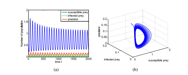
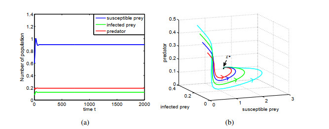
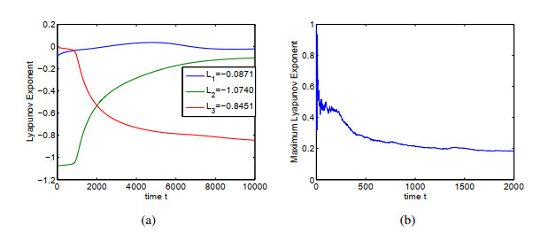
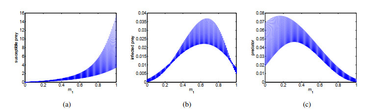
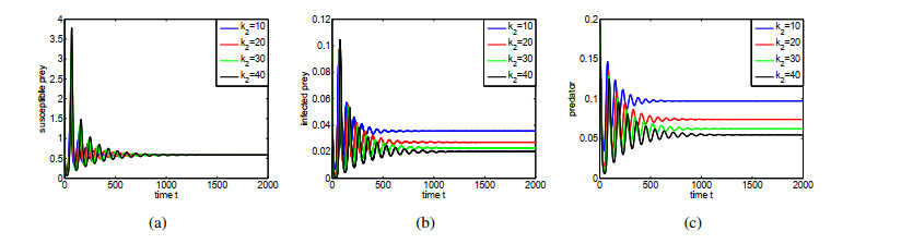
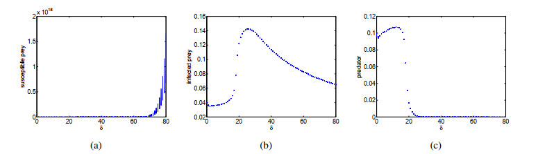
In this article, a delayed predator-prey system with fear effect, disease and herd behavior in prey incorporating refuge is established. Firstly, the positiveness and boundedness of the solutions is proved, and the basic reproduction number $ R_0 $ is calculated. Secondly, by analyzing the characteristic equations of the system, the local asymptotic stability of the equilibria is discussed. Then taking time delay as the bifurcation parameters, the existence of Hopf bifurcation of the system at the positive equilibrium is given. Thirdly, the global asymptotic stability of the equilibria is discussed by constructing a suitable Lyapunov function. Next, the direction of Hopf bifurcation and the stability of the periodic solution are analyzed based on the center manifold theorem and normal form theory. What's more, the impact of the prey refuge, fear effect and capture rate on system is given. Finally, some numerical simulations are performed to verify the correctness of the theoretical results.
- fear effect,
- time delay,
- Hopf bifurcation,
- global stability
Citation: San-Xing Wu, Xin-You Meng. Dynamics of a delayed predator-prey system with fear effect, herd behavior and disease in the susceptible prey[J]. AIMS Mathematics, 2021, 6(4): 3654-3685. doi: 10.3934/math.2021218

Related Papers:

Abstract

In this article, a delayed predator-prey system with fear effect, disease and herd behavior in prey incorporating refuge is established. Firstly, the positiveness and boundedness of the solutions is proved, and the basic reproduction number $ R_0 $ is calculated. Secondly, by analyzing the characteristic equations of the system, the local asymptotic stability of the equilibria is discussed. Then taking time delay as the bifurcation parameters, the existence of Hopf bifurcation of the system at the positive equilibrium is given. Thirdly, the global asymptotic stability of the equilibria is discussed by constructing a suitable Lyapunov function. Next, the direction of Hopf bifurcation and the stability of the periodic solution are analyzed based on the center manifold theorem and normal form theory. What's more, the impact of the prey refuge, fear effect and capture rate on system is given. Finally, some numerical simulations are performed to verify the correctness of the theoretical results.

References

[1]	A. J. Lotka, Elements of physical biology, Williams & Wilkins Company, Baltimore, 1925.
[2]	V. Volterra, Variations and fluctuations of the number of individuals in animal species living together, ICES. J. Mar. Sci., 3 (1928), 3-51. doi: 10.1093/icesjms/3.1.3
[3]	J. E. Cohen, Infectious diseases of humans: Dynamics and control, J. Am. Med. Assoc., 268 (1992), 3381. doi: 10.1001/jama.1992.03490230111047
[4]	J. Chattopadhyay, O. Arino, A predator-prey model with disease in the prey, Nonlinear Anal. Theor., 36 (1999) 747-766. doi: 10.1016/S0362-546X(98)00126-6
[5]	E. Beltrami, T. O. Carroll, Modeling the role of viral disease in recurrent phytoplankton blooms, J. Math. Biol., 32 (1994) 857-863. doi: 10.1007/BF00168802
[6]	Y. G. Wang, Y. N. Li, W. S. Wang, Analysis of a prey-predator model with time delay and disease in prey (Chinese), Math. Pract. Theo., 17 (2016) 284-288.
[7]	L. S. Wang, R. Xu, G. H. Feng, Modelling and analysis of an eco-epidemiological model with time delay and stage structure, J. Appl. Math. Comput., 50 (2016), 175-197. doi: 10.1007/s12190-014-0865-3
[8]	B. W. Li, Z. W. Li, B. S. Chen, G. Wang, Hopf bifurcation analysis of a predator-prey biological economic system with nonselective harvesting, Discrete Dyn. Nat. Soc., 2015 (2015), 1-10. doi: 10.1155/2015/264321
[9]	X. Y. Meng, N. N. Qin, H. F. Huo, Dynamics of a food chain model with two infected predators, Int. J. Bifurcat. Chaos, 2021, doi: 10.1142/S021812742150019X.
[10]	F. Dai, B. Liu, Optimal control problem for a general reaction-diffusion eco-epidemiological model with disease in prey, Appl. Math. Model., 88 (2020), 1-20. doi: 10.1016/j.apm.2020.06.040
[11]	X. Y. Meng, H. F. Huo, X. B. Zhang, Stability and global Hopf bifurcation in a Leslie-Gower predator-prey model with stage structure for prey, J. Appl. Math. Comput., 60 (2019) 1-25. doi: 10.1007/s12190-018-1201-0
[12]	M. Cai, S. L. Yan, Z. J. Du, Positive periodic solutions of an eco-epidemic model with Crowley-Martin type functional response and disease in the prey, Qual. Theor. Dyn. Syst., 19 (2020), 1-20. doi: 10.1007/s12346-019-00337-5
[13]	C. C. Zhu, J. Zhu, Dynamic analysis of a delayed COVID-19 epidemic with home quarantine in temporal-spatial heterogeneous via global exponential attractor method, Chaos Soliton. Fract., 143 (2020), 1-15. doi: 10.1016/j.chaos.2020.110546
[14]	F. Fausto, E. Cuevas, A. Valdivia, A. Gonzalez, A global optimization algorithm inspired in the behavior of selfish herds, Biosystems, 160 (2017), 39-55. doi: 10.1016/j.biosystems.2017.07.010
[15]	W. B. Yang, Existence and asymptotic behavior of solutions for a mathematical ecology model with herd behavior, Math. Method. Appl. Sci., 43 (2020), 5629-5644. doi: 10.1002/mma.6301
[16]	D. Manna, A. Maiti, G. P. Samanta, Analysis of a predator-prey model for exploited fish populations with schooling behavior, Appl. Math. Comput., 317 (2018), 35-48. doi: 10.1016/j.amc.2017.08.052
[17]	S. Belvisi, E. Venturino, An ecoepidemic model with diseased predators and prey group defense, Simul. Model. Pract. Th., 34 (2013), 144-155. doi: 10.1016/j.simpat.2013.02.004
[18]	S. Djilali, Impact of prey herd shape on the predator-prey interaction, Chaos Soliton. Fract., 120 (2019), 139-148. doi: 10.1016/j.chaos.2019.01.022
[19]	S. Saha, G. P. Samanta, Analysis of a predator-prey model with herd behavior and disease in prey incorporating prey refuge, Int. J. Biomath., 12 (2019), 1-18. doi: 10.1142/S1793524519500074
[20]	S. Creel, D. Christianson, Relationships between direct predation and risk effects, Trends Ecol. Evol., 23 (2008), 194-201. doi: 10.1016/j.tree.2007.12.004
[21]	M. Clinchy, M. J. Sheriff, L. Y. Zanette, Predator-induced stress and the ecology of fear, Funct. Ecol., 27 (2013), 56-65. doi: 10.1111/1365-2435.12007
[22]	X. Y. Wang, L. Zanette, X. F. Zou, Modelling the fear effect in predator-prey interactions, J. Math. Biol., 73 (2016), 1179-1204. doi: 10.1007/s00285-016-0989-1
[23]	X. Y. Wang, X. F. Zou, Modeling the fear effect in predator-prey interactions with adaptive avoidance of predators, B. Math. Biol., 79 (2017), 1325-1359. doi: 10.1007/s11538-017-0287-0
[24]	A. Kumar, B. Dubey, Modeling the effect of fear in a prey-predator system with prey refuge and gestation delay, Int. J. Bifurcat. Chaos, 29 (2019), 1950195. doi: 10.1142/S0218127419501955
[25]	Z. L. Zhu, R. X. Wu, L. Y. Lai, X. Q. Yu, The influence of fear effect to the Lotka-Volterra predator-prey system with predator has other food resource, Adv. Differ. Equ., 2020 (2020), 1-13. doi: 10.1186/s13662-019-2438-0
[26]	Y. Huang, Z. Zhu, Z. Li, Modeling the Allee effect and fear effect in predator-prey system incorporating a prey refuge, Adv. Differ. Equ., 2020 (2020), 1-13. doi: 10.1186/s13662-019-2438-0
[27]	S. Devi, Effects of prey refuge on a ratio-dependent predator-prey model with stage-structure of prey population, Appl. Math. Model., 37 (2013), 4337-4349. doi: 10.1016/j.apm.2012.09.045
[28]	Q. Zhu, H. Q. Peng, X. X. Zheng, H. F. Xiao, Bifurcation analysis of a stage-structured predator-prey model with prey refuge, Discrete Cont. Dyn. Syst, 12 (2019), 2195-2209. doi: 10.3934/dcdss.2019141
[29]	Y. Z. Bai, Y. Y. Li, Stability and Hopf bifurcation for a stage-structured predator-prey model incorporating refuge for prey and additional food for predator, Adv. Differ. Equ., 2019 (2019), 1-20. doi: 10.1186/s13662-018-1939-6
[30]	H. S. Zhang, Y. L. Cai, S. M. Fu, W. M. Wang, Impact of the fear effect in a prey-predator model incorporating a prey refuge, Appl. Math. Comput., 356 (2019), 328-337. doi: 10.1016/j.amc.2019.03.034
[31]	D. Mukherjee, C. Maji, Bifurcation analysis of a Holling type II predator-prey model with refuge, Chinese J. Phys., 65 (2020), 153-162. doi: 10.1016/j.cjph.2020.02.012
[32]	W. J. Lu, Y. H. Xia, Y. Z. Bai, Periodic solution of a stage-structured predator-prey model incorporating prey refuge, Math. Biosci. Eng., 17 (2020), 3160-3174. doi: 10.3934/mbe.2020179
[33]	Y. Kuang, Delay Differential Equations with Applications in Population Dynamics, London, Academic Press, 1993.
[34]	B. Mukhopadhyay, R. Bhattacharyya, Dynamics of a delay-diffusion prey-predator model with disease in the prey, J. Appl. Math. Comput., 17 (2005), 361-377. doi: 10.1007/BF02936062
[35]	X. Y. Meng, H. F. Huo, X. B. Zhang, H. Xiang, Stability and Hopf bifurcation in a three-species system with feedback delays, Nonlinear Dynam., 64 (2011), 349-364. doi: 10.1007/s11071-010-9866-4
[36]	X. Y. Meng, J. G. Wang, Dynamical analysis of a delayed diffusive predator-prey model with schooling behavior and Allee effect, J. Biolog. Dyn., 14 (2020), 826-848. doi: 10.1080/17513758.2020.1850892
[37]	D. F. Duan, B. Niu, J. J. Wei, Hopf-Hopf bifurcation and chaotic attractors in a delayed diffusive predator-prey model with fear effect, Chaos Soliton. Fract., 123 (2019), 206-216. doi: 10.1016/j.chaos.2019.04.012
[38]	Z. W. Xiao, Z. Li, Z. L. Zhu, F. D. Chen, Hopf bifurcation and stability in a {B}eddington-{D}e{A}ngelis predator-prey model with stage structure for predator and time delay incorporating prey refuge, Open Math., 17 (2019) 141-159. doi: 10.1515/math-2019-0014
[39]	D. P. Hu, Y. Y. Li, M. Liu, Y. Z. Bai, Stability and Hopf bifurcation for a delayed predator-prey model with stage structure for prey and Ivlev type functional response, Nonlinear Dynam., 99 (2020), 3323-3350. doi: 10.1007/s11071-020-05467-z
[40]	X. Y. Meng, J. Li, Dynamical behavior of a delayed prey-predator-scavenger system with fear effect and linear harvesting, Int. J. Biomath., doi: 10.1142/S1793524521500248.
[41]	N. Bairagi, P. K. Roy, J. Chattopadhyay, Role of infection on the stability of a predator-prey system with several response functionsa comparative study, J. Theor. Biol., 248 (2007), 10-25. doi: 10.1016/j.jtbi.2007.05.005
[42]	C. S. Holling, The functional response of predators to prey density and its role in mimicry and population dynamics, Memo. Entomologi. Soci. Cana., 97 (1965), 5-60. doi: 10.4039/entm9745fv
[43]	J. R. Beddington, Mutual interference between parasites or predators and its effect on searching efficiency, J. Anim. Ecol., 44 (1975), 331-340. doi: 10.2307/3866
[44]	P. H. Crowley, E. K. Martin, Functional responses and interference within and between year classes of a dragonfly population, J. N. Am. Benthol. Soc., 8 (1989), 211-221. doi: 10.2307/1467324
[45]	F. A. Rihan, C. Rajivganthi, Dynamics of fractional-order delay differential model of prey-predator system with Holling-type III and infection among predators, Chaos Soliton. Fract., 141 (2020), 110365. doi: 10.1016/j.chaos.2020.110365
[46]	P. Dreessche, J. Watmough, Reproduction numbers and sub-threshold endemic equilibria for compartmental models of disease transmission, Math. Biosci., 180 (2002), 29-48. doi: 10.1016/S0025-5564(02)00108-6
[47]	Y. L. Song, J. J. Wei, Bifurcation analysis for Chen's system with delayed feedback and its application to control of chaos, Chaos Soliton. Fract., 22 (2004), 75-91. doi: 10.1016/j.chaos.2003.12.075
[48]	B. D. Hassard, N. D. Kazarinoff, Y. H, Theory and Applications of Hopf Bifurcation, Cambridge, Cambridge University Press, 1981. doi: 10.1090/conm/445
[49]	Z. D. Zhang, Q. S. Bi, Bifurcation in a piecewise linear circuit with switching boundaries, Int. J. Bifurcat. Chaos, 22 (2012), 1250034. doi: 10.1142/S0218127412500344
[50]	J. P. LaSalle, The Stability of Dynamical Systems, Philadephia, Society for Industrial & Applied Mathematics, 1976.
[51]	K. Manna, S. P. Chakrabarty, Global stability of one and two discrete delay models for chronic hepatitis B infection with HBV DNA-containing capsids, Comput. Appl. Math., 36 (2017), 525-536. doi: 10.1007/s40314-015-0242-3
[52]	A. Wolf, J. B. Swift, H. L. Swinney, J. A. Vastano, Determining Lyapounov exponents from a time series, Physica D, 16 (1985), 285-317. doi: 10.1016/0167-2789(85)90011-9
[53]	R. K. Goodrich, A riesz representation theorem, P. Am. Math. Soc., 24 (1970), 629-636. doi: 10.1090/S0002-9939-1970-0415386-2
[54]	F. A. Rihan, Sensitivity analysis for dynamic systems with time-lags, J. Comput. Appl. Math., 151 (2003), 445-462. doi: 10.1016/S0377-0427(02)00659-3
[55]	M. A. Imron, A. Gergs, U. Berger, Structure and sensitivity analysis of individual-based predator-prey models, Reliab. Eng. Syst. Safe., 107 (2012), 71-81. doi: 10.1016/j.ress.2011.07.005

Reader Comments

Your name:*

Email:*
© 2021 the Author(s), licensee AIMS Press. This is an open access article distributed under the terms of the Creative Commons Attribution License (http://creativecommons.org/licenses/by/4.0)