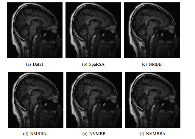
In this study, we develop a nonmonotone variable metric Barzilai-Borwein method for minimizing the sum of a smooth function and a convex, possibly nondifferentiable, function. At each step, the descent direction is obtained by taking the difference between the minimizer of the scaling proximal function and the current iteration point. An adaptive nonmonotone line search is proposed for determining the step length along this direction. We also show that the limit point of the iterates sequence is a stationary point. Numerical results with parallel magnetic resonance imaging, Poisson, and Cauchy noise deblurring demonstrate the effectiveness of the new algorithm.
Citation: Xiao Guo, Chuanpei Xu, Zhibin Zhu, Benxin Zhang. Nonmonotone variable metric Barzilai-Borwein method for composite minimization problem[J]. AIMS Mathematics, 2024, 9(6): 16335-16353. doi: 10.3934/math.2024791
In this study, we develop a nonmonotone variable metric Barzilai-Borwein method for minimizing the sum of a smooth function and a convex, possibly nondifferentiable, function. At each step, the descent direction is obtained by taking the difference between the minimizer of the scaling proximal function and the current iteration point. An adaptive nonmonotone line search is proposed for determining the step length along this direction. We also show that the limit point of the iterates sequence is a stationary point. Numerical results with parallel magnetic resonance imaging, Poisson, and Cauchy noise deblurring demonstrate the effectiveness of the new algorithm.

| [1] |
E. J. Candes, J. Romberg, T. Tao, Robust uncertainty principles: exact signal reconstruction from highly incomplete frequency information, IEEE Trans. Inf. Theory, 52 (2006), 489–509. https://doi.org/10.1109/TIT.2005.862083 doi: 10.1109/TIT.2005.862083

|
| [2] |
E. T. Hale, W. Yin, Y. Zhang, Fixed-point continuation for $l_1$-minimization: methodology and convergence, SIAM J. Optim., 19 (2008), 1107–1130. https://doi.org/10.1137/070698920 doi: 10.1137/070698920
|
| [3] |
Y. Li, C. Li, W. Yang, W. Zhang, A new conjugate gradient method with a restart direction and its application in image restoration, AIMS Math., 8 (2023), 28791–28807. https://doi.org/10.3934/math.20231475 doi: 10.3934/math.20231475
|
| [4] |
A. Chambolle, An algorithm for total variation minimization and applications, J. Math. Imag. Vis., 20 (2004), 89–97. https://doi.org/10.1023/B:JMIV.0000011325.36760.1e doi: 10.1023/B:JMIV.0000011325.36760.1e
|
| [5] |
L. Rudin, S. Osher, E. Fatemi, Nonlinear total variation based noise removal algorithms, Phys. D, 60 (1992), 259–268. https://doi.org/10.1016/0167-2789(92)90242-F doi: 10.1016/0167-2789(92)90242-F
|
| [6] |
N. Artsawang, Accelerated preconditioning Krasnosel'skii-Mann method for efficiently solving monotone inclusion problems, AIMS Math., 8 (2023), 28398–28412. https://doi.org/10.3934/math.20231453 doi: 10.3934/math.20231453
|
| [7] |
P. H. Calamai, J. J. Moré, Projeeted gradient methods for linearly constralned problems, Math. Program., 39 (1987), 93–116. https://doi.org/10.1007/BF02592073 doi: 10.1007/BF02592073
|
| [8] | D. P. Bertsekas, Nonlinear programming, Athena scientific, Belmont, 1999. |
| [9] |
J. Barzilai, J. M. Borwein, Two point step size gradient methods, IMA J. Numer. Anal., 8 (1988), 141–148. https://doi.org/10.1093/imanum/8.1.141 doi: 10.1093/imanum/8.1.141
|
| [10] |
E. G. Birgin, J. M. Martínez, M. Raydan, Nonmonotone spectral projected gradient methods on convex sets, SIAM J. Optim., 10 (2000), 1196–1211. https://doi.org/10.1137/S1052623497330963 doi: 10.1137/S1052623497330963
|
| [11] |
Y. H. Dai, R. Fletcher, Projected Barzilai-Borwein methods for large-scale box-constrained quadratic programming, Numer. Math., 100 (2005), 21–47. https://doi.org/10.1007/s00211-004-0569-y doi: 10.1007/s00211-004-0569-y
|
| [12] |
B. Zhang, Z. Zhu, S. Li, A modified spectral conjugate gradient projection algorithm for total variation image restoration, Appl. Math. Lett., 27 (2014), 26–35. https://doi.org/10.1016/j.aml.2013.08.006 doi: 10.1016/j.aml.2013.08.006
|
| [13] |
I. Daubechies, M. Defrise, C. De Mol, An iterative thresholding algorithm for linear inverse problems with a sparsity constraint, Commun. Pure Appl. Math., 57 (2004), 1413–1457. https://doi.org/10.1002/cpa.20042 doi: 10.1002/cpa.20042
|
| [14] |
A. Beck, M. Teboulle, A fast iterative shrinkage-thresholding algorithm for linear inverse problems, SIAM J. Imag. Sci., 2 (2009), 183–202. https://doi.org/10.1137/080716542 doi: 10.1137/080716542
|
| [15] |
E. T. Hale, W. Yin, Y. Zhang, Fixed-point continuation applied to compressed sensing: implementation and numerical experiments, J. Comput. Math., 28 (2010), 170–194. https://doi.org/10.4208/jcm.2009.10-m1007 doi: 10.4208/jcm.2009.10-m1007
|
| [16] |
S. J. Wright, R. D. Nowak, T. Figueiredo, Sparse reconstruction by separable approximation, IEEE Trans. Signal Process., 57 (2009), 2479–2493. https://doi.org/10.1109/TSP.2009.2016892 doi: 10.1109/TSP.2009.2016892
|
| [17] |
W. W. Hager, D. T. Phan, H. Zhang, Gradient-based methods for sparse recovery, SIAM J. Imag. Sci., 4 (2011), 146–165. https://doi.org/10.1137/090775063 doi: 10.1137/090775063
|
| [18] |
Y. Huang, H. Liu, A Barzilai-Borwein type method for minimizing composite functions, Numer. Algorithms, 69 (2015), 819–838. https://doi.org/10.1007/s11075-014-9927-8 doi: 10.1007/s11075-014-9927-8
|
| [19] |
W. Cheng, Z. Chen, D. Li, Nonmonotone spectral gradient method for sparse recovery, Inverse Probl. Imag., 9 (2015), 815–833. https://doi.org/10.3934/ipi.2015.9.815 doi: 10.3934/ipi.2015.9.815
|
| [20] |
Y. Xiao, S. Y. Wu, L. Qi, Nonmonotone Barzilai-Borwein gradient algorithm for $l_1$-regularized nonsmooth minimization in compressive sensing, J. Sci. Comput., 61 (2014), 17–41. https://doi.org/10.1007/s10915-013-9815-8 doi: 10.1007/s10915-013-9815-8
|
| [21] |
P. Tseng, S. Yun, A coordinate gradient descent method for nonsmooth separable minimization, Math. Program., 117 (2009), 387–423. https://doi.org/10.1007/s10107-007-0170-0 doi: 10.1007/s10107-007-0170-0
|
| [22] |
E. Chouzenoux, J. C. Pesquet, A. Repetti, Variable metric forward-backward algorithm for minimizing the sum of a differentiable function and a convex function, J. Optim. Theory Appl., 162 (2014), 107–132. https://doi.org/10.1007/s10957-013-0465-7 doi: 10.1007/s10957-013-0465-7
|
| [23] |
P. L. Combettes, B. C. Vû, Variable metric forward-backward splitting with applications to monotone inclusions in duality, Optimization, 63 (2014), 1289–1318. https://doi.org/10.1080/02331934.2012.733883 doi: 10.1080/02331934.2012.733883
|
| [24] |
S. Bonettini, I. Loris, F. Porta, M. Prato, Variable metric inexact line-search-based methods for nonsmooth optimization, SIAM J. Optim., 26 (2016), 891–921. https://doi.org/10.1137/15M1019325 doi: 10.1137/15M1019325
|
| [25] |
S. Rebegoldi, L. Calatroni, Scaled, inexact and adaptive generalized FISTA for strongly convex optimization, SIAM J. Optim., 32 (2022), 2428–2459. https://doi.org/10.1137/21M1391699 doi: 10.1137/21M1391699
|
| [26] |
S.Bonettini, M. Prato, S. Rebegoldi, A new proximal heavy ball inexact line-search algorithm, Comput. Optim. Appl., 2024. https://doi.org/10.1007/s10589-024-00565-9 doi: 10.1007/s10589-024-00565-9
|
| [27] |
, S. Bonettini, P. Ochs, M. Prato, S. Rebegoldi, An abstract convergence framework with application to inertial inexact forward-backward methods, Comput. Optim. Appl., 84 (2023), 319–362. https://doi.org/10.1007/s10589-022-00441-4 doi: 10.1007/s10589-022-00441-4
|
| [28] |
H. Liu, T. Wang, Z. Liu, A nonmonotone accelerated proximal gradient method with variable stepsize strategy for nonsmooth and nonconvex minimization problems, J. Glob. Optim., 2024. https://doi.org/10.1007/s10898-024-01366-4 doi: 10.1007/s10898-024-01366-4
|
| [29] |
Y. Chen, W. W. Hager, M. Yashtini, X. Ye, H. Zhang, Bregman operator splitting with variable stepsize for total variation image reconstruction, Comput. Optim. Appl., 54 (2013), 317–342. https://doi.org/10.1007/s10589-012-9519-2 doi: 10.1007/s10589-012-9519-2
|
| [30] |
Y. Chen, W. W. Hager, F. Huang, D. T. Phan, X. Ye, W. Yin, Fast algorithms for image reconstruction with application to partially parallel MR imaging, SIAM J. Imag. Sci., 5 (2012), 90–118. https://doi.org/10.1137/100792688 doi: 10.1137/100792688
|
| [31] |
S. Bonettini, M. Prato, New convergence results for the scaled gradient projection method, Inverse Probl., 31 (2015), 095008. https://doi.org/10.1088/0266-5611/31/9/095008 doi: 10.1088/0266-5611/31/9/095008
|
| [32] |
F. Porta, M. Prato, L. Zanni, A new steplength selection for scaled gradient methods with application to image deblurring, J. Sci. Comput., 65 (2015), 895–919. https://doi.org/10.1007/s10915-015-9991-9 doi: 10.1007/s10915-015-9991-9
|
| [33] |
L. Grippo, F. Lampariello, S. Lucidi, A nonmonotone line search technique for Newton's method, SIAM J. Numer. Anal., 23 (1986), 707–716. https://doi.org/10.1137/0723046 doi: 10.1137/0723046
|
| [34] |
K. Amini, M. Ahookhosh, H. Nosratipour, An inexact line search approach using modified nonmonotone strategy for unconstrained optimization, Numer. Algorithms, 66 (2014), 49–78. https://doi.org/10.1007/s11075-013-9723-x doi: 10.1007/s11075-013-9723-x
|
| [35] | R. T. Rockafellar, Convex analysis, Princeton University Press, 2015. |
| [36] |
Y. Ouyang, Y. Chen, G. Lan, J. E. Pasiliao, An accelerated linearized alternating direction method of multipliers, SIAM J. Imag. Sci., 8 (2015), 644–681. https://doi.org/10.1137/14095697X doi: 10.1137/14095697X
|
| [37] |
X. Ye, Y. Chen, F. Huang, Computational acceleration for MR image reconstruction in partially parallel imaging, IEEE Trans. Med. Imag., 30 (2011), 1055–1063. https://doi.org/10.1109/TMI.2010.2073717 doi: 10.1109/TMI.2010.2073717
|
| [38] |
S. Bonettini, I. Loris, F. Porta, M. Prato, S. Rebegoldi, On the convergence of a linesearch based proximal-gradient method for nonconvex optimization, Inverse Probl., 33 (2017), 055005. https://doi.org/10.1088/1361-6420/aa5bfd doi: 10.1088/1361-6420/aa5bfd
|
| [39] |
S. Bonettini, M. Prato, S. Rebegoldi, Convergence of inexact forward-backward algorithms using the forward-backward envelope, SIAM J. Optim., 30 (2020), 3069–3097. https://doi.org/10.1137/19M1254155 doi: 10.1137/19M1254155
|
| [40] |
M. K. Riahi, I. A. Qattan, On the convergence rate of Fletcher-Reeves nonlinear conjugate gradient methods satisfying strong Wolfe conditions: application to parameter identification in problems governed by general dynamics, Math. Methods Appl. Sci., 45 (2022), 3644–3664. https://doi.org/10.1002/mma.8009 doi: 10.1002/mma.8009
|
| [41] |
X. Li, Q. L. Dong, A. Gibali, PMiCA-Parallel multi-step inertial contracting algorithm for solving common variational inclusions, J. Nonlinear Funct. Anal., 2022 (2022), 7. https://doi.org//10.23952/jnfa.2022.7 doi: 10.23952/jnfa.2022.7
|
| [42] |
L. O. Jolaoso, Y. Shehu, J. Yao, R. Xu, Double inertial parameters forward-backward splitting method: applications to compressed sensing, image processing, and SCAD penalty problems, J. Nonlinear Var. Anal., 7 (2023), 627–646. https://doi.org/10.23952/jnva.7.2023.4.10 doi: 10.23952/jnva.7.2023.4.10
|


Figures(6) / Tables(3)

Xiao Guo, Chuanpei Xu, Zhibin Zhu, Benxin Zhang. Nonmonotone variable metric Barzilai-Borwein method for composite minimization problem[J]. AIMS Mathematics, 2024, 9(6): 16335-16353. doi: 10.3934/math.2024791


 DownLoad: