Proportional fractional Dirac dynamic system

Tuba Gulsen; Emrah Yilmaz; Ayse Çiğdem Yar; Tuba Gulsen; Emrah Yilmaz; Ayse Çiğdem Yar

doi:10.3934/math.2024487

AIMS Mathematics

2024, Volume 9, Issue 4: 9951-9968. doi: 10.3934/math.2024487

Previous Article Next Article

Research article Special Issues

Proportional fractional Dirac dynamic system

1.
Department of Mathematics, Faculty of Science, Firat University, Elazığ, Turkey
2.
Department of Mathematics, Institute of Science, Firat University, Elazığ, Turkey

Received: 22 January 2024 Revised: 04 March 2024 Accepted: 07 March 2024 Published: 12 March 2024
MSC : 35Q41, 34N05, 26A33

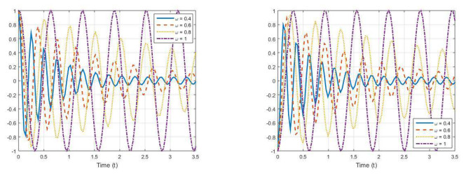
In this study, considering the proportional fractional derivative, which is a generalization of the conformable fractional derivative, we provided some important spectral properties such as the reality of eigenvalues, the orthogonality of eigenfunctions, the self-adjointness of the operator, the asymptotic estimations of eigenfunctions, and Picone's identity for a proportional Dirac system on an arbitrary time scale. We also presented graphics representing the eigenfunctions of the Dirac system on a time scale, produced by taking advantage of the proportional fractional derivative with some special cases. The main purpose of presenting these graphics was to examine the effect of the proportional fractional derivative on the Dirac system on a time scale, as well as the effect of the eigenvalues, which are meaningful for the subject we were studying for the solution functions.
- Dirac operator,
- time scales,
- proportional fractional derivative
Citation: Tuba Gulsen, Emrah Yilmaz, Ayse Çiğdem Yar. Proportional fractional Dirac dynamic system[J]. AIMS Mathematics, 2024, 9(4): 9951-9968. doi: 10.3934/math.2024487

Related Papers:

Abstract

In this study, considering the proportional fractional derivative, which is a generalization of the conformable fractional derivative, we provided some important spectral properties such as the reality of eigenvalues, the orthogonality of eigenfunctions, the self-adjointness of the operator, the asymptotic estimations of eigenfunctions, and Picone's identity for a proportional Dirac system on an arbitrary time scale. We also presented graphics representing the eigenfunctions of the Dirac system on a time scale, produced by taking advantage of the proportional fractional derivative with some special cases. The main purpose of presenting these graphics was to examine the effect of the proportional fractional derivative on the Dirac system on a time scale, as well as the effect of the eigenvalues, which are meaningful for the subject we were studying for the solution functions.

References

[1]	R. K. Amirov, B. Keskin, G. Özkan, Direct and inverse problems for the Dirac operator with a spectral parameter linearly contained in a boundary condition, Ukr. Math. Zhurnal, 61 (2009), 1365–1379.
[2]	A. Kablan, T. Özden, A Dirac system with transmission condition and eigenparameter in boundary condition, Abstr. Appl. Anal., 2013 (2013), 395457. http://dx.doi.org/10.1155/2013/395457 doi: 10.1155/2013/395457
[3]	B. Keskin, A. S. Ozkan, Inverse spectral problems for Dirac operator with eigenvalue dependent boundary and jump conditions, Acta Math. Hung., 130 (2011), 309–320. http://dx.doi.org/10.1007/s10474-010-0052-4 doi: 10.1007/s10474-010-0052-4
[4]	B. P. Allahverdiev, H. Tuna, One-dimensional conformable fractional Dirac system, Bol. Soc. Mat. Mex., 26 (2020), 121–146. http://dx.doi.org/10.1007/s40590-019-00235-5 doi: 10.1007/s40590-019-00235-5
[5]	B. P. Allahverdiev, H. Tuna, Conformable fractional dynamic Dirac system, Ann. Univ. Ferrara., 69 (2023), 203–218. http://dx.doi.org/10.1007/s11565-022-00412-x doi: 10.1007/s11565-022-00412-x
[6]	T. Abdeljewad, On conformable fractional calculus, J. Comput. Appl. Math., 279 (2015), 57–66. http://dx.doi.org/10.1016/j.cam.2014.10.016 doi: 10.1016/j.cam.2014.10.016
[7]	N. Benkhettou, A. M. C. B. da Cruz, D. F. M. Torres, A fractional calculus on arbitrary time scales: Fractional differentiation and fractional integration, Signal Process., 107 (2015), 230–237. http://dx.doi.org/10.1016/j.sigpro.2014.05.026 doi: 10.1016/j.sigpro.2014.05.026
[8]	N. Benkhettou, S. Hassani, D. F. M. Torres, A conformable fractional calculus on arbitrary time scales, J. King Saud Univ. Sci., 28 (2016), 93–98. http://dx.doi.org/10.1016/j.jksus.2015.05.003 doi: 10.1016/j.jksus.2015.05.003
[9]	T. Gulsen, E. Yilmaz, S. Goktas, Conformable fractional Dirac system on time scales, J. Inequal. Appl., 161 (2017). http://dx.doi.org/10.1186/s13660-017-1434-8 doi: 10.1186/s13660-017-1434-8
[10]	T. Gülșen, E. Yilmaz, H. Kemaloğlu, Conformable fractional Sturm-Liouville equation and some existence results on time scales, Turk. J. Math., 42 (2018), 1348–1360. http://dx.doi.org/10.3906/mat-1704-120 doi: 10.3906/mat-1704-120
[11]	U. Katugampola, A new fractional derivative with classical properties, arXiv Preprint, 2014. http://dx.doi.org/10.48550/arXiv.1410.6535
[12]	R. Khalil, M. Al Horani, A. Yousef, M. Sababheh, A new definition of fractional derivative, J. Comput. Appl. Math., 264 (2014), 57–66. http://dx.doi.org/10.1016/j.cam.2014.01.002 doi: 10.1016/j.cam.2014.01.002
[13]	M. D. Ortigueira, J. T. Machado, What is a fractional derivative? J. Comput. Phys., 293 (2015), 4–13. http://dx.doi.org/10.1016/j.jcp.2014.07.019 doi: 10.1016/j.jcp.2014.07.019
[14]	E. Yilmaz, T. Gulsen, E. S. Panakhov, Existence results for a conformable type Dirac system on time scales in quantum physics, Appl. Comput. Math., 21 (2022), 279–291. http://dx.doi.org/10.30546/1683-6154.21.3.2022.279 doi: 10.30546/1683-6154.21.3.2022.279
[15]	R. Agarwal, M. Bohner, D. O'Regan, A. Peterson, Dynamic equations on time scales: A survey, J. Comput. Appl. Math., 141 (2002), 1–26. http://dx.doi.org/10.1016/S0377-0427(01)00432-0 doi: 10.1016/S0377-0427(01)00432-0
[16]	B. Aulbach, S. Hilger. A unified approach to continuous and discrete dynamics, Colloquia Mathematica Sociefatis János Bolyai, Amsterdam: North-Holland, 53 (1990), 37–56.
[17]	M. Bohner, A. Peterson, Dynamic equations on time scales: An introduction with applications, 1 Eds., Boston: Springer Science & Business Media, 2001. http://doi.org/10.1007/978-1-4612-0201-1
[18]	M. Bohner, A. Peterson, Advances in dynamic equations on time scales, 1 Eds., Boston: Birkhauser, 2004. http://doi.org/10.1007/978-0-8176-8230-9
[19]	M. Bohner, G. Svetlin, Multivariable dynamic calculus on time scales, 1 Eds., Cham: Springer, 2016. http://doi.org/10.1007/978-3-319-47620-9
[20]	S. Hilger, Analysis on measure chains a unified approach to continuous and discrete calculus, Results Math., 18 (1990), 18–56. http://dx.doi.org/10.1007/BF03323153 doi: 10.1007/BF03323153
[21]	M. Bohner, T. Li, Kamenev-type criteria for nonlinear damped dynamic equations, Sci. China Math., 58 (2015), 1445–1452. http://dx.doi.org/10.1007/s11425-015-4974-8 doi: 10.1007/s11425-015-4974-8
[22]	S. Ahmad, A. Ullah, K. Shah, A. Akgül, Computational analysis of the third order dispersive fractional PDE under exponential-decay and Mittag-Leffler type kernels, Numer. Meth. Part. D. E., 39 (2023), 4533–4548. http://dx.doi.org/10.1002/num.22627 doi: 10.1002/num.22627
[23]	K. Shah, T. Abdeljawad, Study of a mathematical model of COVID-19 outbreak using some advanced analysis, Wave. Random Complex, 2022 (2022), 1–18. http://dx.doi.org/10.1080/17455030.2022.2149890 doi: 10.1080/17455030.2022.2149890
[24]	I. Ahmad, K. Shah, G. ur Rahman, D. Baleanu, Stability analysis for a nonlinear coupled system of fractional hybrid delay differential equations, Math. Method. Appl. Sci., 43 (2020), 8669–8682. http://dx.doi.org/10.1002/mma.6526 doi: 10.1002/mma.6526
[25]	A. Ullah, T. Abdeljawad, S. Ahmad, K. Shah, Study of a fractional-order epidemic model of childhood diseases, J. Funct. Space., 2020 (2020), 5895310. http://dx.doi.org/10.1155/2020/5895310 doi: 10.1155/2020/5895310
[26]	A. Columbu, S. Frassu, G. Viglialoro, Properties of given and detected unbounded solutions to a class of chemotaxis models, Stud. Appl. Math., 151 (2023), 1349–1379. http://dx.doi.org/10.48550/arXiv.2303.15039 doi: 10.48550/arXiv.2303.15039
[27]	T. Li, S. Frassu, G. Viglialoro, Combining effects ensuring boundedness in an attraction-repulsion chemotaxis model with production and consumption, Z. Angew. Math. Phys., 109 (2023), 1–21. http://dx.doi.org/10.1007/s00033-023-01976-0 doi: 10.1007/s00033-023-01976-0
[28]	C. Zhang, R. P. Agarwal, M. Bohner, T. Li, Oscillation of fourth-order delay dynamic equations, Sci. China Math., 58 (2015), 143–160. http://dx.doi.org/10.1007/s11425-014-4917-9 doi: 10.1007/s11425-014-4917-9
[29]	D. R. Anderson, D. J. Ulness, Newly defined conformable derivatives, Adv. Dynam. Syst. Appl., 10 (2015), 109–137.
[30]	Y. Li, K. H. Ang, G. C. Chong, PID control system analysis and design, IEEE Control Syst. Mag., 26 (2006), 32–41. http://dx.doi.org/10.1109/MCS.2006.1580152 doi: 10.1109/MCS.2006.1580152
[31]	M. R. S. Rahmat, A new definition of conformable fractional derivative on arbitrary time scales, Adv. Differential Equ., 2019 (2019), 1–16. http://dx.doi.org/10.1186/s13662-019-2294-y doi: 10.1186/s13662-019-2294-y
[32]	D. R. Anderson, S. G. Georgiev, Conformable dynamic equations on time scales, 1 Eds., CRC Press, 2020. http://dx.doi.org/10.1201/9781003057406
[33]	D. Hinton, Sturm's 1836 oscillation results evolution of the Sturm-Liouville theory, 1 Eds., Basel: Birkhäuser, 2005. http://dx.doi.org/10.1007/3-7643-7359-8-1
[34]	Z. S. Aliyev, H. S. Rzayeva, Oscillation properties of the eigenvector-functions of the one-dimensional Dirac's canonical system, Proc. Inst. Math. Mech., 40 (2014), 36–48.

Reader Comments

Your name:*

Email:*
© 2024 the Author(s), licensee AIMS Press. This is an open access article distributed under the terms of the Creative Commons Attribution License (http://creativecommons.org/licenses/by/4.0)