A co-infection with Covid-19 and dengue fever has had worse outcomes due to high mortality rates and longer stays either in isolation or at hospitals. This poses a great threat to a country's economy. To effectively deal with these threats, comprehensive approaches to prevent and control Covid-19/dengue fever co-infections are desperately needed. Thus, our focus is to formulate a new co-infection fractional model with the Atangana-Baleanu derivative to suggest effective and feasible approaches to restrict the spread of co-infection. In the first part of this paper, we present Covid-19 and dengue fever sub-models, as well as the co-infection model that is locally asymptotically stable when the respective reproduction numbers are less than unity. We establish the existence and uniqueness results for the solutions of the co-infection model. We extend the model to include a vaccination compartment for the Covid-19 vaccine to susceptible individuals and a treatment compartment to treat dengue-infected individuals as optimal control strategies for disease control. We outline the fundamental requirements for the fractional optimal control problem and illustrate the optimality system for the co-infection model using Pontraygin's principle. We implement the Toufik-Atangana approximating scheme to simulate the optimality system. The simulations show the effectiveness of the implemented strategy in determining optimal vaccination and treatment rates that decrease the cost functional to a minimum, thus significantly decreasing the number of infected humans and vectors. Additionally, we visualize a meaningful decrease in infection cases with an increase in the memory index. The findings of this study will provide reasonable disease control suggestions to regions facing Covid-19 and dengue fever co-infection.
Citation: Asma Hanif, Azhar Iqbal Kashif Butt, Tariq Ismaeel. Fractional optimal control analysis of Covid-19 and dengue fever co-infection model with Atangana-Baleanu derivative[J]. AIMS Mathematics, 2024, 9(3): 5171-5203. doi: 10.3934/math.2024251
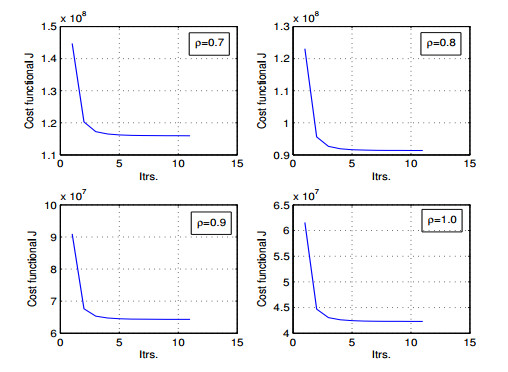
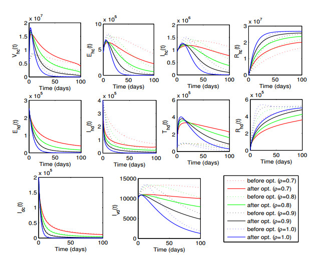
A co-infection with Covid-19 and dengue fever has had worse outcomes due to high mortality rates and longer stays either in isolation or at hospitals. This poses a great threat to a country's economy. To effectively deal with these threats, comprehensive approaches to prevent and control Covid-19/dengue fever co-infections are desperately needed. Thus, our focus is to formulate a new co-infection fractional model with the Atangana-Baleanu derivative to suggest effective and feasible approaches to restrict the spread of co-infection. In the first part of this paper, we present Covid-19 and dengue fever sub-models, as well as the co-infection model that is locally asymptotically stable when the respective reproduction numbers are less than unity. We establish the existence and uniqueness results for the solutions of the co-infection model. We extend the model to include a vaccination compartment for the Covid-19 vaccine to susceptible individuals and a treatment compartment to treat dengue-infected individuals as optimal control strategies for disease control. We outline the fundamental requirements for the fractional optimal control problem and illustrate the optimality system for the co-infection model using Pontraygin's principle. We implement the Toufik-Atangana approximating scheme to simulate the optimality system. The simulations show the effectiveness of the implemented strategy in determining optimal vaccination and treatment rates that decrease the cost functional to a minimum, thus significantly decreasing the number of infected humans and vectors. Additionally, we visualize a meaningful decrease in infection cases with an increase in the memory index. The findings of this study will provide reasonable disease control suggestions to regions facing Covid-19 and dengue fever co-infection.

| [1] | World Health Organization, Epidemiological bulletin WHO health emergencies programme WHO regional office for south-east Asia, 8 Eds., 2023. Available from: https://iris.who.int/handle/10665/372269 |
| [2] |
S. Naseer, S. Khalid, S. Parveen, K. Abbass, H. Song, M. V. Achim, COVID-19 outbreak: Impact on global economy, Front. Public Health, 10 (2023), 1009393. https://doi.org/10.3389/fpubh.2022.1009393 doi: 10.3389/fpubh.2022.1009393

|
| [3] |
Y. Shang, H. Li, R. Zhang, Effects of Pandemic outbreak on economies: Evidence from business history context, Front. Public Health, 9 (2021), 632043. https://doi.org/10.3389/fpubh.2021.632043 doi: 10.3389/fpubh.2021.632043
|
| [4] |
S. Murthy, C. D. Gomersall, R. A. Fowler, Care for critically ill patients with Covid-19, JAMA, 323 (2020), 1499–1500. https://doi.org/10.1001/jama.2020.3633 doi: 10.1001/jama.2020.3633
|
| [5] |
H. S. Rodrigues, M. T. T. Monteiro, D. F. M. Torres, Sensitivity analysis in a dengue epidemiological model, Conf. Pap. Math., 2013 (2013), 721406. https://doi.org/10.1155/2013/721406 doi: 10.1155/2013/721406
|
| [6] | World Health Organization, Dengue guidelines, for diagnosis, treatment, prevention and control, 2009. Available from: https://www.who.int/publications-detail-redirect/9789241547871 |
| [7] |
M. Verduyn, N. Allou, V. Gazaille, M. Andre, T. Desroche, M. C. Jaffar et al., Co-infection of dengue and Covid-19: A case report, PLoS Negl. Trop. Dis., 14 (2020), e0008476. https://doi.org/10.1371/journal.pntd.0008476 doi: 10.1371/journal.pntd.0008476
|
| [8] | S. Masyeni, M. S. Santoso, P. D. Widyaningsih, D. G. W. Asmara, F. Nainu, H. Harapan, et al., Serological cross-reaction and coinfection of dengue and COVID-19 in Asia: Experience from Indonesia, Int. J. Infect. Dis., 102 (2021), 152–154. https://doi.org/10.1016j.ijid.2020.10.043 |
| [9] |
L. Lansbury, B. Lim, V. Baskaran, W. S. Lim, Co-infections in people with Covid-19: A systematic review and meta-analysis, J. infect., 81 (2020), 266–275. https://doi.org/10.1016/j.jinf.2020.05.046 doi: 10.1016/j.jinf.2020.05.046
|
| [10] |
A. A. Malibari, F. Al-Husayni, A. Jabri, A. Al-Amri, M. Alharbi, A patient with Dengue Fever and COVID-19: coinfection or not? Cureus, 12 (2020), e11955. https://doi.org/10.7759/cureus.11955 doi: 10.7759/cureus.11955
|
| [11] |
A. Saddique, M. S. Rana, M. M. Alam, A. Ikram, M. Usman, M. Salman, et al., Emergence of co-infection of COVID-19 and dengue: A serious public health threat, J. Infect., 81 (2020), e16–e18. https://doi.org/10.1016/j.jinf.2020.08.009 doi: 10.1016/j.jinf.2020.08.009
|
| [12] |
M. I. H. Hussein, A. A. D. Albashir, O. A. M. A. Elawad, A. Homeida, Malaria and COVID-19: Unmasking their ties, Malaria J., 19 (2020), 457. https://doi.org/10.1186/s12936-020-03541-w doi: 10.1186/s12936-020-03541-w
|
| [13] |
K. Sverdrup, S. J. Kimmerle, P. Berg, Computational investigation of the stability and dissolution of nanobubbles, Appl. Math. Model., 49 (2017), 199–219. https://doi.org/10.1016/j.apm.2017.05.006 doi: 10.1016/j.apm.2017.05.006
|
| [14] |
M. Farman, A. Akgül, M. T. Tekin, M. M. Akram, A. Ahmad, E. E. Mahmoud, et al., Fractal fractional-order derivative for HIV/AIDS model with Mittag-Leffler kernel, Alex. Eng. J., 61 (2022), 10965–10980. https://doi.org/10.1016/j.aej.2022.04.030 doi: 10.1016/j.aej.2022.04.030
|
| [15] |
S. Ahmad, A. Ullah, A. Akgül, D. Baleanu, Analysis of the fractional tumour-immune-vitamins model with Mittag-Leffler kernel, Results Phys., 19 (2020), 103559. https://doi.org/10.1016/j.rinp.2020.103559 doi: 10.1016/j.rinp.2020.103559
|
| [16] |
Y. Sabbar, A. Din, D. Kiouach, Influence of fractal-fractional differentiation and independent quadratic Levy jumps on the dynamics of a general epidemic model with vaccination strategy, Chaos Solitons Fractals, 171 (2023), 113434. https://doi.org/10.1016/j.chaos.2023.113434 doi: 10.1016/j.chaos.2023.113434
|
| [17] |
A. I. K. Butt, Atangana-Baleanu fractional dynamics of predictive whooping Cough model with optimal control analysis, Symmetry, 15 (2023), 1773. https://doi.org/10.3390/sym15091773 doi: 10.3390/sym15091773
|
| [18] |
B. Fatima, M. Yavuz, M Ur Rahman, A. Althobaiti, S. Althobaiti, Predictive modeling and control strategies for the transmission of middle east respiratory syndrome coronavirus, Math. Comput. Appl., 28 (2023), 98. https://doi.org/10.3390/mca28050098 doi: 10.3390/mca28050098
|
| [19] |
A. Hanif, A. I. K. Butt, Atangana-Baleanu fractional dynamics of dengue fever with optimal control strategies, AIMS Mathematics, 8 (2023), 15499–15535. https://doi.org/10.3934/math.2023791 doi: 10.3934/math.2023791
|
| [20] |
A. Omame, D. Okuonghae, A co-infection model for oncogenic Human papillomavirus and tuberculosis with optimal control and cost-effectiveness analysis, Optim. Control. Appl. Methods, 42 (2021), 1081–1101. https://doi.org/10.1002/oca.2717 doi: 10.1002/oca.2717
|
| [21] |
Y. Guo, T. Li, Fractional-order modeling and optimal control of a new online game addiction model based on real data, Commun. Nonlinear Sci. Numer. Simul., 121 (2023), 107221. https://doi.org/10.1016/j.cnsns.2023.107221 doi: 10.1016/j.cnsns.2023.107221
|
| [22] |
D. Baleanu, F. A. Ghassabzade, J. J. Nieto, A. Jajarmi, On a new and generalized fractional model for a real cholera outbreak, Alex. Eng. J., 61 (2022), 9175–9186. https://doi.org/10.1016/j.aej.2022.02.054 doi: 10.1016/j.aej.2022.02.054
|
| [23] |
B. Razia, T. Osman, H. Khan, G. Haseena, A. Khan, A fractional order Zika virus model with Mittag-Leffler kernel, Chaos Solitons Fractals, 146 (2021), 110898. https://doi.org/10.1016/j.chaos.2021.110898 doi: 10.1016/j.chaos.2021.110898
|
| [24] |
A. Atangana, I. Koca, Chaos in a simple nonlinear system with Atangana-Baleanu derivative with fractional order, Chaos Solitons Fractals, 89 (2016), 447–454. https://doi.org/10.1016/j.chaos.2016.02.012 doi: 10.1016/j.chaos.2016.02.012
|
| [25] |
A. I. K. Butt, W. Ahmad, M. Rafiq, N. Ahmad, M. Imran, Optimally analyzed fractional Coronavirus model with Atangana–Baleanu derivative, Results Phys., 53 (2023), 106929. https://doi.org/10.1016/j.rinp.2023.106929 doi: 10.1016/j.rinp.2023.106929
|
| [26] |
M. Caputo, M. Fabrizio, A new definition of fractional derivative without singular kernel, Progr. Fract. Differ. Appl., 1 (2015), 73–85. http://doi.org/10.12785/pfda/010201 doi: 10.12785/pfda/010201
|
| [27] |
D. Baleanu, A. Jajarmi, H. Mohammadi, S. Rezapour, A new study on the mathematical modelling of human liver with Caputo-Fabrizio fractional derivative, Chaos Solitons Fractals, 134 (2020), 109705. https://doi.org/10.1016/j.chaos.2020.109705 doi: 10.1016/j.chaos.2020.109705
|
| [28] |
T. Khan, R. Ullah, G. Zaman, J. Alzabut, A mathematical model for the dynamics of SARS-CoV-2 virus using the Caputo-Fabrizio operator, Math. Biosci. Eng., 18 (2021), 6095–6116. https://doi.org/10.3934/mbe.2021305 doi: 10.3934/mbe.2021305
|
| [29] |
A. I. K. Butt, M. Imran, S. Batool, M. Al Nuwairan, Theoretical analysis of a COVID-19 CF-fractional model to optimally control the spread of pandemic, Symmetry, 15 (2023), 380. https://doi.org/10.3390/sym15020380 doi: 10.3390/sym15020380
|
| [30] | A. A. Kilbas, H. M. Srivastava, J. J. Trujillo, Theory and applications of fractional differential equations, Elsevier Science, 2006. |
| [31] |
A. Atangana, D. Balneau, New fractional derivative with nonlocal and nonsingular kernel: Theory and application to heat transfer model, Thermal Sci., 20 (2016), 763–769. http://doi.org/10.2298/TSCI160111018A doi: 10.2298/TSCI160111018A
|
| [32] |
M. A. Al Shorbagy, M. Ur Rahman, Y. Karaca, A computational analysis fractional complex-order values by ABC operator and Mittag-Leffler Kernel modeling, Fractals, 31 (2023), 2340164. https://doi.org/10.1142/S0218348X23401643 doi: 10.1142/S0218348X23401643
|
| [33] |
P. Liu, Mati ur Rahman, A. Din, Fractal fractional based transmission dynamics of COVID-19 epidemic model, Comput. Methods Biomec. Biomed. Eng., 25 (2022), 1852–1869. https://doi.org/10.1080/10255842.2022.2040489 doi: 10.1080/10255842.2022.2040489
|
| [34] |
A. Hanif, A. I. K. Butt, W. Ahmad, Numerical approach to solve Caputo‐Fabrizio‐fractional model of corona pandemic with optimal control design and analysis, Math. Methods Appl. Sci., 46 (2023), 9751–9782. https://doi.org/10.1002/mma.9085 doi: 10.1002/mma.9085
|
| [35] |
A. Hanif, A. I. K. Butt, S. Ahmad, R. U. Din, M. Inc, A new fuzzy fractional order model of transmission of Covid-19 with quarantine class, Eur. Phys. J. Plus, 136 (2021), 1179. https://doi.org/10.1140/epjp/s13360-021-02178-1 doi: 10.1140/epjp/s13360-021-02178-1
|
| [36] |
A. I. K. Butt, M. Rafiq, W. Ahmad, N. Ahmad, Implementation of computationally efficient numerical approach to analyze a Covid-19 pandemic model, Alex. Eng. J., 69 (2023), 341–362. https://doi.org/10.1016/j.aej.2023.01.052 doi: 10.1016/j.aej.2023.01.052
|
| [37] |
M. L. Diagne, H. Rwezaura, S. Y. Tchoumi, J. M. Tchuenche, A mathematical model of Covid-19 with vaccination and treatment, Comput. Math. Methods Med., 2021 (2021), 1250129. https://doi.org/10.1155/2021/1250129 doi: 10.1155/2021/1250129
|
| [38] |
A. I. K. Butt, W. Ahmad, M. Rafiq, N. Ahmad, M. Imran, Computationally efficient optimal control analysis for the mathematical model of Coronavirus pandemic, Expert Syst. Appl., 234 (2023), 121094. https://doi.org/10.1016/j.eswa.2023.121094 doi: 10.1016/j.eswa.2023.121094
|
| [39] |
K. Diethelm, A fractional calculus based model for the simulation of an outbreak of dengue fever, Nonlinear Dynam., 71 (2013), 613–619. https://doi.org/10.1007/s11071-012-0475-2 doi: 10.1007/s11071-012-0475-2
|
| [40] |
Y. Chu, S. Sultana, S. Rashid, M. S. Alharthi, Dynamical analysis of the stochastic COVID-19 model using piecewise differential equation technique, Comput. Model. Eng. Sci., 137 (2023), 2427–2464. https://doi.org/10.32604/cmes.2023.028771 doi: 10.32604/cmes.2023.028771
|
| [41] |
Y. Chu, S. Rashid, A. O. Akdemir, A. Khalid, D. Baleanu, B. R. Al-Sinan, et al., Predictive dynamical modeling and stability of the equilibria in a discrete fractional difference COVID-19 epidemic model, Results Phys., 49 (2023), 106467. https://doi.org/10.1016/j.rinp.2023.106467 doi: 10.1016/j.rinp.2023.106467
|
| [42] |
T. Li, Y. Guo, Modeling and optimal control of mutated COVID-19 (Delta strain) with imperfect vaccination, Chaos Solitons Fractals, 156 (2022), 111825. https://doi.org/10.1016/j.chaos.2022.111825 doi: 10.1016/j.chaos.2022.111825
|
| [43] |
A. I. K. Butt, M. Imran, B. A. McKinney, S. Batool, H. Aftab, Mathematical and stability analysis of dengue-malaria co-infection with disease control strategies, Mathematics, 11 (2023), 4600. https://doi.org/10.3390/math11224600 doi: 10.3390/math11224600
|
| [44] |
E. Mtisi, H. Rwezaura, J. M. Tchuenche, A mathematical analysis of malaria and tuberculosis co-dynamics, Discrete Contin. Dyn. Syst. Ser. B, 12 (2009), 827–864. https://doi.org/10.3934/dcdsb.2009.12.827 doi: 10.3934/dcdsb.2009.12.827
|
| [45] |
A. Omame, M. Abbas, C. P. Onyenegecha, A fractional-order model for Covid-19 and tuberculosis co-infection using Atangana-Baleanu derivative, Chaos Solitons Fractals, 153 (2001), 111486. https://doi.org/10.1016/j.chaos.2021.111486 doi: 10.1016/j.chaos.2021.111486
|
| [46] |
A. Omame, H. Rwezaura, M. L. Diagne, S. C. Inyama, J. M. Tchuenche, COVID-19 and dengue co-infection in Brazil: Optimal control and cost-effectiveness analysis, Eur. Phys. J. Plus, 136 (2021), 1090. https://doi.org/10.1140/epjp/s13360-021-02030-6 doi: 10.1140/epjp/s13360-021-02030-6
|
| [47] |
A. Atangana, D. Baleanu, New fractional derivatives with nonlocal and non-singular kernel: Theory and applications to heat transfer model, Therm Sci., 20 (2016), 763–769. http://dx.doi.org/10.2298/TSCI160111018A doi: 10.2298/TSCI160111018A
|
| [48] |
J. K. K. Asamoah, Fractal fractional model and numerical scheme based on Newton polynomial for Q fever disease under Atangana-Baleanu derivative, Results Phys., 34 (2022), 105189. https://doi.org/10.1016/j.rinp.2022.105189 doi: 10.1016/j.rinp.2022.105189
|
| [49] | G. Birkhoff, G. C. Rota, Ordinary differential equations, 4 Eds., John Wiley & Sons, 1991. |
| [50] |
C. M. A. Pinto, J. A. T. Machado, Fractional model for malaria transmission under control strategies, Comput. Math. Appl., 66 (2013), 908–916. https://doi.org/10.1016/j.camwa.2012.11.017 doi: 10.1016/j.camwa.2012.11.017
|
| [51] |
E. Mtisi, H. Rwezaura, J.M. Tchuenche, A mathematical analysis of malaria and tuberculosis co-dynamics, Discrete Contin. Dyn. Syst. Ser. B, 12 (2009), 827–864. https://doi.org/10.3934/dcdsb.2009.12.827 doi: 10.3934/dcdsb.2009.12.827
|
| [52] |
M. Toufik, A. Atangana, New numerical approximation of fractional derivative with non-local and non-singular kernel: Application to chaotic models, Eur. Phys. J. Plus, 132 (2017), 444. https://doi.org/10.1140/epjp/i2017-11717-0 doi: 10.1140/epjp/i2017-11717-0
|
| [53] |
R. Kamocki, Pontryagin maximum principle for fractional ordinary optimal control problems, Math. Methods Appl. Sci., 37 (2014), 1668–1686. https://doi.org/10.1002/mma.2928 doi: 10.1002/mma.2928
|
| [54] | S. Lenhart, J. T. Workman, Optimal control applied to biological models, CRC Press, 2007. |
| [55] |
H. M. Ali, F. L. Pereira, S. M. A. Gama, A new approach to the Pontryagin maximum principle for nonlinear fractional optimal control problems, Math. Methods Appl. Sci., 39 (2016), 3640–3649. https://doi.org/10.1002/mma.3811 doi: 10.1002/mma.3811
|
Figures(6) / Tables(1)

Asma Hanif, Azhar Iqbal Kashif Butt, Tariq Ismaeel. Fractional optimal control analysis of Covid-19 and dengue fever co-infection model with Atangana-Baleanu derivative[J]. AIMS Mathematics, 2024, 9(3): 5171-5203. doi: 10.3934/math.2024251


 DownLoad: