In recent years, augmented reality has emerged as an emerging technology with huge potential in image-guided surgery, and in particular, its application in brain tumor surgery seems promising. Augmented reality can be divided into two parts: hardware and software. Further, artificial intelligence, and deep learning in particular, have attracted great interest from researchers in the medical field, especially for the diagnosis of brain tumors. In this paper, we focus on the software part of an augmented reality scenario. The main objective of this study was to develop a classification technique based on a deep belief network (DBN) and a softmax classifier to (1) distinguish a benign brain tumor from a malignant one by exploiting the spatial heterogeneity of cancer tumors and homologous anatomical structures, and (2) extract the brain tumor features. In this work, we developed three steps to explain our classification method. In the first step, a global affine transformation is preprocessed for registration to obtain the same or similar results for different locations (voxels, ROI). In the next step, an unsupervised DBN with unlabeled features is used for the learning process. The discriminative subsets of features obtained in the first two steps serve as input to the classifier and are used in the third step for evaluation by a hybrid system combining the DBN and a softmax classifier. For the evaluation, we used data from Harvard Medical School to train the DBN with softmax regression. The model performed well in the classification phase, achieving an improved accuracy of 97.2%.
Citation: Karim Gasmi, Ahmed Kharrat, Lassaad Ben Ammar, Ibtihel Ben Ltaifa, Moez Krichen, Manel Mrabet, Hamoud Alshammari, Samia Yahyaoui, Kais Khaldi, Olfa Hrizi. Classification of MRI brain tumors based on registration preprocessing and deep belief networks[J]. AIMS Mathematics, 2024, 9(2): 4604-4631. doi: 10.3934/math.2024222
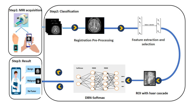
In recent years, augmented reality has emerged as an emerging technology with huge potential in image-guided surgery, and in particular, its application in brain tumor surgery seems promising. Augmented reality can be divided into two parts: hardware and software. Further, artificial intelligence, and deep learning in particular, have attracted great interest from researchers in the medical field, especially for the diagnosis of brain tumors. In this paper, we focus on the software part of an augmented reality scenario. The main objective of this study was to develop a classification technique based on a deep belief network (DBN) and a softmax classifier to (1) distinguish a benign brain tumor from a malignant one by exploiting the spatial heterogeneity of cancer tumors and homologous anatomical structures, and (2) extract the brain tumor features. In this work, we developed three steps to explain our classification method. In the first step, a global affine transformation is preprocessed for registration to obtain the same or similar results for different locations (voxels, ROI). In the next step, an unsupervised DBN with unlabeled features is used for the learning process. The discriminative subsets of features obtained in the first two steps serve as input to the classifier and are used in the third step for evaluation by a hybrid system combining the DBN and a softmax classifier. For the evaluation, we used data from Harvard Medical School to train the DBN with softmax regression. The model performed well in the classification phase, achieving an improved accuracy of 97.2%.

| [1] |
K. Klinker, M. Wiesche, H. Krcmar, Digital transformation in health care: Augmented reality for hands-free service innovation, Inform. Syst. Front., 22 (2020), 1419–1431. https://doi.org/10.1007/s10796-019-09937-7 doi: 10.1007/s10796-019-09937-7

|
| [2] | C. Jung, G. Wolff, B. Wernly, R. R. Bruno, M. Franz, P. C. Schulze, et al., Virtual and augmented reality in cardiovascular care: state-of-the-art and future perspectives, Cardiovascular Imag., 15 (2022), 519–532. https://www.jacc.org/doi/abs/10.1016/j.jcmg.2021.08.017 |
| [3] |
F. Davnall, C. S. Yip, G. Ljungqvist, M. Selmi, F. Ng, B. Sanghera, et al., Assessment of tumor heterogeneity: An emerging imaging tool for clinical practice?, Insights Imaging, 3 (2012), 573–589. https://doi.org/10.1007/s13244-012-0196-6 doi: 10.1007/s13244-012-0196-6
|
| [4] |
S. Bauer, R. Wiest, L. P. Nolte, M. Reyes, A survey of mri-based medical image analysis for brain tumor studies, Phys. Med. Biol., 58 (2013), R97. https://doi.org/10.1088/0031-9155/58/13/r97 doi: 10.1088/0031-9155/58/13/r97
|
| [5] | A. Madani, M. Moradi, A. Karargyris, T. Syeda-Mahmood, Semi-supervised learning with generative adversarial networks for chest x-ray classification with ability of data domain adaptation, in: 2018 IEEE 15th International symposium on biomedical imaging (ISBI 2018), IEEE, 2018, 1038–1042. 10.1109/ISBI.2018.8363749 |
| [6] |
A. Van Opbroek, M. A. Ikram, M. W. Vernooij, M. De Bruijne, Transfer learning improves supervised image segmentation across imaging protocols, IEEE T. Med. Imaging, 34 (2014), 1018–1030. https://doi.org/10.1109/tmi.2014.2366792 doi: 10.1109/tmi.2014.2366792
|
| [7] |
N. Varuna Shree, T. Kumar, Identification and classification of brain tumor mri images with feature extraction using dwt and probabilistic neural network, Brain Informatics, 5 (2018), 23–30. https://doi.org/10.1007/s40708-017-0075-5 doi: 10.1007/s40708-017-0075-5
|
| [8] |
O. Hrizi, K. Gasmi, I. Ben Ltaifa, H. Alshammari, H. Karamti, M. Krichen, et al., Tuberculosis disease diagnosis based on an optimized machine learning model, J. Healthc. Eng., 2022 (2022), https://doi.org/10.1155/2022/8950243 doi: 10.1155/2022/8950243
|
| [9] | G. B. Abdennour, K. Gasmi, R. Ejbali, Ensemble learning model for medical text classification, in: International Conference on Web Information Systems Engineering, Springer, 2023, 3–12. https://doi.org/10.1007/978-981-99-7254-8_1 |
| [10] |
A. K. Attili, A. Schuster, E. Nagel, J. H. Reiber, R. J. Van der Geest, Quantification in cardiac mri: Advances in image acquisition and processing, Int. J. Cardiovas. Imag., 26 (2010), 27–40. https://doi.org/10.1007/s10554-009-9571-x doi: 10.1007/s10554-009-9571-x
|
| [11] |
L. Cai, J. Gao, D. Zhao, A review of the application of deep learning in medical image classification and segmentation, Ann. Transl. Med., 8 (2020). https://doi.org/10.21037/atm.2020.02.44 doi: 10.21037/atm.2020.02.44
|
| [12] | R. Li, W. Zhang, H. I. Suk, L. Wang, J. Li, D. Shen, et al., Deep learning based imaging data completion for improved brain disease diagnosis, in: International conference on medical image computing and computer-assisted intervention, Springer, 2014, 305–312. https://doi.org/10.1007/978-3-319-10443-0_39 |
| [13] |
J. De Fauw, J. R. Ledsam, B. Romera-Paredes, S. Nikolov, N. Tomasev, S. Blackwell, et al., Clinically applicable deep learning for diagnosis and referral in retinal disease, Nat. Med., 24 (2018), 1342–1350. https://doi.org/10.1038/s41591-018-0107-6 doi: 10.1038/s41591-018-0107-6
|
| [14] |
A. Ramcharan, P. McCloskey, K. Baranowski, N. Mbilinyi, L. Mrisho, M. Ndalahwa, et al., A mobile-based deep learning model for cassava disease diagnosis, Front. Plant sci., 10 (2019), 272. https://doi.org/10.3389/fpls.2019.00272 doi: 10.3389/fpls.2019.00272
|
| [15] |
K. Gasmi, I. B. Ltaifa, G. Lejeune, H. Alshammari, L. B. Ammar, M. A. Mahmood, Optimal deep neural network-based model for answering visual medical question, Cybern. Syst., (2021), 1–22. https://doi.org/10.1080/01969722.2021.2018543 doi: 10.1080/01969722.2021.2018543
|
| [16] | P. Sapra, R. Singh, S. Khurana, Brain tumor detection using neural network, Int. J. Sci. Modern Eng., (2013) 2319–6386. https://www.ijisme.org/wp-content/uploads/papers/v1i9/I0425081913.pdf |
| [17] | K. Simonyan, A. Zisserman, Very deep convolutional networks for large-scale image recognition, arXiv preprint arXiv: 1409.1556 (2014). |
| [18] |
M. Rizwan, A. Shabbir, A. R. Javed, M. Shabbir, T. Baker, D. A.-J. Obe, Brain tumor and glioma grade classification using gaussian convolutional neural network, IEEE Access, 10 (2022), 29731–29740. https://doi.org/10.1109/access.2022.3153108 doi: 10.1109/access.2022.3153108
|
| [19] |
A. Krizhevsky, I. Sutskever, G. E. Hinton, Imagenet classification with deep convolutional neural networks, Adv. Neural Inf. Process. Syst., 25 (2012). https://doi.org/10.1145/3065386 doi: 10.1145/3065386
|
| [20] |
S. C. Turaga, J. F. Murray, V. Jain, F. Roth, M. Helmstaedter, K. Briggman, et al, Convolutional networks can learn to generate affinity graphs for image segmentation, Neural Comput., 22 (2010), 511–538. https://doi.org/10.1162/neco.2009.10-08-881 doi: 10.1162/neco.2009.10-08-881
|
| [21] |
A. Kharrat, M. Neji, A system for brain image segmentation and classification based on three-dimensional convolutional neural network, Comput. Sist., 24 (2020), 1617–1626. https://doi.org/10.13053/cys-24-4-3058 doi: 10.13053/cys-24-4-3058
|
| [22] |
A. Rehman, S. Naz, M. I. Razzak, F. Akram, M. Imran, A deep learning-based framework for automatic brain tumors classification using transfer learning, Circ. Syst. Signal Pr., 39 (2020), 757–775. https://doi.org/10.1007/s00034-019-01246-3 doi: 10.1007/s00034-019-01246-3
|
| [23] |
M. Krichen, Convolutional Neural Networks: A Survey, Computers, 12 (2023), 151. https://doi.org/10.3390/computers12080151 doi: 10.3390/computers12080151
|
| [24] | N. Montemurro, S. Condino, M. Carbone, N. Cattari, R. D'Amato, F. Cutolo, et al., Brain tumor and augmented reality: New technologies for the future, 2022. https://doi.org/10.3390/ijerph19106347 |
| [25] |
M. Krichen, A. J. Maâlej, M. Lahami, A model-based approach to combine conformance and load tests: An ehealth case study, Int. J. Critical Computer-Based Syst., 8 (2018), 282–310. https://doi.org/10.1504/ijccbs.2018.096437 doi: 10.1504/ijccbs.2018.096437
|
| [26] |
P. E. Pelargos, D. T. Nagasawa, C. Lagman, S. Tenn, J. V. Demos, S. J. Lee, et al., Utilizing virtual and augmented reality for educational and clinical enhancements in neurosurgery, J. Clin. Neurosci., 35 (2017), 1–4. https://doi.org/10.1016/j.jocn.2016.09.002 doi: 10.1016/j.jocn.2016.09.002
|
| [27] |
Q. Shan, T. E. Doyle, R. Samavi, M. Al-Rei, Augmented reality based brain tumor 3d visualization, Procedia Comput. Sci., 113 (2017), 400–407. https://doi.org/10.1016/j.procs.2017.08.356 doi: 10.1016/j.procs.2017.08.356
|
| [28] |
R. Tagaytayan, A. Kelemen, C. Sik-Lanyi, Augmented reality in neurosurgery, Arch. Med. Sci., 14 (2018), 572–578. https://doi.org/10.5114/aoms.2016.58690 doi: 10.5114/aoms.2016.58690
|
| [29] |
C. Lee, G. K. C. Wong, Virtual reality and augmented reality in the management of intracranial tumors: A review, J. Clin. Neurosci., 62 (2019), 14–20. https://doi.org/10.1016/j.jocn.2018.12.036 doi: 10.1016/j.jocn.2018.12.036
|
| [30] |
H. Greenspan, B. Van Ginneken, R. M. Summers, Guest editorial deep learning in medical imaging: Overview and future promise of an exciting new technique, IEEE T. Med. Imaging, 35 (2016), 1153–1159. https://doi.org/10.1109/tmi.2016.2553401 doi: 10.1109/tmi.2016.2553401
|
| [31] |
A. S. Lundervold, A. Lundervold, An overview of deep learning in medical imaging focusing on mri, Z. Medizinische Phys., 29 (2019), 102–127. https://doi.org/10.1016/j.zemedi.2018.11.002 doi: 10.1016/j.zemedi.2018.11.002
|
| [32] | G. Tomasila, A. W. R. Emanuel, Mri image processing method on brain tumors: A review, in: AIP Conference Proceedings, volume 2296, AIP Publishing LLC, 2020, 020023. https://doi.org/10.1063/5.0030978 |
| [33] | A. Kharrat, N. Mahmoud, Feature selection based on hybrid optimization for magnetic resonance imaging brain tumor classification and segmentation, Appl. Med. Inf., 41 (2019), 9–23. https://ami.info.umfcluj.ro/index.php/AMI/article/view/648 |
| [34] |
A. Hossain, M. T. Islam, S. K. Abdul Rahim, M. A. Rahman, T. Rahman, H. Arshad, et al., A lightweight deep learning based microwave brain image network model for brain tumor classification using reconstructed microwave brain (rmb) images, Biosensors, 13 (2023), 238. https://doi.org/10.3390/bios13020238 doi: 10.3390/bios13020238
|
| [35] |
B. Pattanaik, K. Anitha, S. Rathore, P. Biswas, P. Sethy, S. Behera, Brain tumor magnetic resonance images classification based machine learning paradigms, Contemporary Oncol., 27 (2022). https://doi.org/10.5114/wo.2023.124612 doi: 10.5114/wo.2023.124612
|
| [36] |
M. Rasool, N. A. Ismail, A. Al-Dhaqm, W. Yafooz, A. Alsaeedi, A novel approach for classifying brain tumours combining a squeezenet model with svm and fine-tuning, Electronics, 12 (2023), 149. https://doi.org/10.3390/electronics12010149 doi: 10.3390/electronics12010149
|
| [37] |
S. Solanki, U. P. Singh, S. S. Chouhan, S. Jain, Brain tumor detection and classification using intelligence techniques: An overview, IEEE Access, 2023). https://doi.org/10.1109/access.2023.3242666 doi: 10.1109/access.2023.3242666
|
| [38] | K. Wisaeng, W. Sa-Ngiamvibool, Brain tumor segmentation using fuzzy otsu threshold morphological algorithm, IAENG Int. J. Appl. Math., 53 (2023), 1–12. |
| [39] | T. Schmah, G. E. Hinton, S. Small, S. Strother, R. Zemel, Generative versus discriminative training of rbms for classification of fmri images, Adv. Neural Inf. Proc. Syst., 21 (2008). http://www.cs.toronto.edu/fritz/absps/fmrinips.pdf |
| [40] | C. Dev, K. Kumar, A. Palathil, T. Anjali, V. Panicker, Machine learning based approach for detection of lung cancer in dicom ct image, in: Ambient Communications and Computer Systems, Springer, 2019, 161–173. https://doi.org/10.1007/978-981-13-5934-7_15 |
| [41] | T. Williams, R. Li, Wavelet pooling for convolutional neural networks, in: International Conference on Learning Representations, 2018, 1. |
| [42] |
E. I. Zacharaki, S. Wang, S. Chawla, D. Soo Yoo, R. Wolf, E. R. Melhem, et al., Classification of brain tumor type and grade using mri texture and shape in a machine learning scheme, Magn. Reson. Med., 62 (2009), 1609–1618. https://doi.org/10.1002/mrm.22147 doi: 10.1002/mrm.22147
|
| [43] | K. Machhale, H. B. Nandpuru, V. Kapur, L. Kosta, Mri brain cancer classification using hybrid classifier (svm-knn), in: 2015 International Conference on Industrial Instrumentation and Control (ICIC), IEEE, 2015, 60–65. https://doi.org/10.1109/iic.2015.7150592 |
| [44] | A. S. Ansari, Numerical simulation and development of brain tumor segmentation and classification of brain tumor using improved support vector machine, Int. J. Intell. Syst. Appl. Eng., 11 (2023), 35–44. https://www.ijisae.org/index.php/IJISAE/article/view/2505 |
| [45] | O. Ariyo, Q. Zhi-guang, L. Tian, Brain mr segmentation using a fusion of k-means and spatial fuzzy c-means, in: 2017 International conference on computer science and application engineering (CSAE 2017), 2017, 863–873. https://doi.org/10.12783/dtcse/csae2017/17565 |
| [46] |
M. Sharif, M. A. Khan, Z. Iqbal, M. F. Azam, M. I. U. Lali, M. Y. Javed, Detection and classification of citrus diseases in agriculture based on optimized weighted segmentation and feature selection, Comput. Electron. Agr., 150 (2018), 220–234. https://doi.org/10.1016/j.compag.2018.04.023 doi: 10.1016/j.compag.2018.04.023
|
| [47] |
P. A. Babu, B. S. Rao, Y. V. B. Reddy, G. R. Kumar, J. N. Rao, S. K. R. Koduru, et al., Optimized cnn-based brain tumor segmentation and classification using artificial bee colony and thresholding, Int. J. Comput. Commun. Control, 18 (2023). https://doi.org/10.15837/ijccc.2023.1.4577 doi: 10.15837/ijccc.2023.1.4577
|
| [48] | M. Sharma, G. Purohit, S. Mukherjee, Information retrieves from brain mri images for tumor detection using hybrid technique k-means and artificial neural network (kmann), in: Networking communication and data knowledge engineering, Springer, 2018, 145–157. https://doi.org/10.1007/978-981-10-4600-1_14 |
| [49] | A. Mikołajczyk, M. Grochowski, Data augmentation for improving deep learning in image classification problem, in: 2018 international interdisciplinary PhD workshop (IIPhDW), IEEE, 2018, 117–122. https://doi.org/10.1109/iiphdw.2018.8388338 |
| [50] |
L. Zhang, X. Wang, D. Yang, T. Sanford, S. Harmon, B. Turkbey, et al., Generalizing deep learning for medical image segmentation to unseen domains via deep stacked transformation, IEEE T. Med. Imaging, 39 (2020), 2531–2540. https://doi.org/10.1109/tmi.2020.2973595 doi: 10.1109/tmi.2020.2973595
|
| [51] |
A. Işın, C. Direkoğlu, M. Şah, Review of mri-based brain tumor image segmentation using deep learning methods, Procedia Comput. Sci., 102 (2016), 317–324. https://doi.org/10.1016/j.procs.2016.09.407 doi: 10.1016/j.procs.2016.09.407
|
| [52] |
N. Varuna Shree, T. Kumar, Identification and classification of brain tumor mri images with feature extraction using dwt and probabilistic neural network, Brain Inform., 5 (2018), 23–30. https://doi.org/10.1007/s40708-017-0075-5 doi: 10.1007/s40708-017-0075-5
|
| [53] |
M. A. Hamid, N. A. Khan, Investigation and classification of mri brain tumors using feature extraction technique, J. Med. Biol. Eng., 40 (2020), 307–317. https://doi.org/10.1007/s40846-020-00510-1 doi: 10.1007/s40846-020-00510-1
|
| [54] |
Y. Chen, H. Jiang, C. Li, X. Jia, P. Ghamisi, Deep feature extraction and classification of hyperspectral images based on convolutional neural networks, IEEE T. Geosci. Remote, 54 (2016), 6232–6251. https://doi.org/10.1109/tgrs.2016.2584107 doi: 10.1109/tgrs.2016.2584107
|
| [55] | X. Yang, Y. Fan, Feature extraction using convolutional neural networks for multi-atlas based image segmentation, in: Medical Imaging 2018: Image Processing, volume 10574, International Society for Optics and Photonics, 2018, 1057439. https://doi.org/10.1117/12.2293876 |
| [56] |
A. M. Hasan, H. A. Jalab, F. Meziane, H. Kahtan, A. S. Al-Ahmad, Combining deep and handcrafted image features for mri brain scan classification, IEEE Access, 7 (2019), 79959–79967. https://doi.org/10.1109/access.2019.2922691 doi: 10.1109/access.2019.2922691
|
| [57] |
H. El Hamdaoui, A. Benfares, S. Boujraf, N. E. H. Chaoui, B. Alami, M. Maaroufi, et al., High precision brain tumor classification model based on deep transfer learning and stacking concepts, Indones. J. Electr. Eng. Comput. Sci., 24 (2021), 167–177. https://doi.org/10.11591/ijeecs.v24.i1.pp167-177 doi: 10.11591/ijeecs.v24.i1.pp167-177
|
| [58] |
A. Khatami, A. Khosravi, T. Nguyen, C. P. Lim, S. Nahavandi, Medical image analysis using wavelet transform and deep belief networks, Expert Syst. Appl., 86 (2017), 190–198. https://doi.org/10.1016/j.eswa.2017.05.073 doi: 10.1016/j.eswa.2017.05.073
|
| [59] |
N. D. G. Carneiro, A. P. Bradley, Automated mass detection from mammograms using deep learning and random forest, International Conference on Digital Image Computing: Techniques and Applications (DICTA), (2016) 1–8. https://doi.org/10.1109/dicta.2015.7371234 doi: 10.1109/dicta.2015.7371234
|
| [60] |
Z. N. Shahweli, Deep belief network for predicting the predisposition to lung cancer in tp53 gene, Iraqi J. Sci., (2020), 171–177. https://doi.org/10.24996/ijs.2020.61.1.19 doi: 10.24996/ijs.2020.61.1.19
|
| [61] | T. Jemimma, Y. J. V. Raj, Brain tumor segmentation and classification using deep belief network, in: 2018 Second International Conference on Intelligent Computing and Control Systems (ICICCS), IEEE, 2018, 1390–1394. https://doi.org/10.1109/iccons.2018.8663207 |
| [62] |
N. Farajzadeh, N. Sadeghzadeh, M. Hashemzadeh, Brain tumor segmentation and classification on mri via deep hybrid representation learning, Expert Syst. Appl., 224 (2023), 119963. https://doi.org/10.1016/j.eswa.2023.119963 doi: 10.1016/j.eswa.2023.119963
|
| [63] |
H. H. Sultan, N. M. Salem, W. Al-Atabany, Multi-classification of brain tumor images using deep neural network, IEEE Access, 7 (2019), 69215–69225. https://doi.org/10.1109/access.2019.2919122 doi: 10.1109/access.2019.2919122
|
| [64] |
M. M. Badža, M. Č. Barjaktarović, Classification of brain tumors from mri images using a convolutional neural network, Appl. Sci., 10 (2020), 1999. https://doi.org/10.3390/app10061999 doi: 10.3390/app10061999
|
| [65] |
A. R. Raju, S. Pabboju, R. R. Rao, Hybrid active contour model and deep belief network based approach for brain tumor segmentation and classification, Sensor Rev., (2019). https://doi.org/10.1108/sr-01-2018-0008 doi: 10.1108/sr-01-2018-0008
|
| [66] | A. Kharrat, M. Néji, Classification of brain tumors using personalized deep belief networks on mrimages: Pdbn-mri, in: Eleventh International Conference on Machine Vision (ICMV 2018), volume 11041, SPIE, 2019, 713–721. https://doi.org/10.1117/12.2522848 |
| [67] |
S. Deepa, J. Janet, S. Sumathi, J. Ananth, Hybrid optimization algorithm enabled deep learning approach brain tumor segmentation and classification using mri, J. Digit. Imaging, 36 (2023), 847–868. https://doi.org/10.1007/s10278-022-00752-2 doi: 10.1007/s10278-022-00752-2
|
| [68] |
B. E. Bejnordi, M. Veta, P. J. Van Diest, B. Van Ginneken, N. Karssemeijer, G. Litjens, et al., Diagnostic assessment of deep learning algorithms for detection of lymph node metastases in women with breast cancer, Jama, 318 (2017), 2199–2210. 10.1001/jama.2017.14585 doi: 10.1001/jama.2017.14585
|
| [69] |
M. F. Alanazi, M. U. Ali, S. J. Hussain, A. Zafar, M. Mohatram, M. Irfan, et al., Brain tumor/mass classification framework using magnetic-resonance-imaging-based isolated and developed transfer deep-learning model, Sensors, 22 (2022), 372. https://doi.org/10.3390/s22010372 doi: 10.3390/s22010372
|
| [70] |
B. B. Avants, C. L. Epstein, M. Grossman, J. C. Gee, Symmetric diffeomorphic image registration with cross-correlation: Evaluating automated labeling of elderly and neurodegenerative brain, Med. Image Anal., 12 (2008), 26–41. https://doi.org/10.1016/j.media.2007.06.004 doi: 10.1016/j.media.2007.06.004
|
| [71] |
M. P. Heinrich, I. J. Simpson, B. W. Papież, M. Brady, J. A. Schnabel, Deformable image registration by combining uncertainty estimates from supervoxel belief propagation, Med. Image Anal., 27 (2016), 57–71. https://doi.org/10.1016/j.media.2015.09.005 doi: 10.1016/j.media.2015.09.005
|
| [72] | A. V. Dalca, G. Balakrishnan, J. Guttag, M. R. Sabuncu, Unsupervised learning for fast probabilistic diffeomorphic registration, in: International Conference on Medical Image Computing and Computer-Assisted Intervention, Springer, 2018, pp. 729–738. https://doi.org/10.1016/j.media.2019.07.006 |
| [73] | G. Balakrishnan, A. Zhao, M. R. Sabuncu, J. Guttag, A. V. Dalca, An unsupervised learning model for deformable medical image registration, in: Proceedings of the IEEE conference on computer vision and pattern recognition, 2018, 9252–9260. https://doi.org/10.1109/cvpr.2018.00964 |
| [74] |
M. Holden, A review of geometric transformations for nonrigid body registration, IEEE T. Med. Imaging, 27 (2007), 111–128. https://doi.org/10.1109/tmi.2007.904691 doi: 10.1109/tmi.2007.904691
|
| [75] | A. V. Dalca, G. Balakrishnan, J. Guttag, M. R. Sabuncu, Unsupervised learning for fast probabilistic diffeomorphic registration, in: International Conference on Medical Image Computing and Computer-Assisted Intervention, Springer, 2018, 729–738. https://doi.org/10.1016/j.media.2019.07.006 |
| [76] | P. Viola, M. Jones, Rapid object detection using a boosted cascade of simple features, in: Proceedings of the 2001 IEEE computer society conference on computer vision and pattern recognition. CVPR 2001, volume 1, Ieee, 2001, Ⅰ–Ⅰ. https://doi.org/10.1109/cvpr.2001.990517 |
| [77] |
G. E. Hinton, T. J. Sejnowski, Learning and relearning in boltzmann machines, Parallel distributed processing: Explorations in the microstructure of cognition, 1 (1986), 2. https://doi.org/10.7551/mitpress/3349.003.0005 doi: 10.7551/mitpress/3349.003.0005
|
| [78] |
M. Zambra, A. Testolin, M. Zorzi, A developmental approach for training deep belief networks, Cogn. Comput., 15 (2023), 103–120. https://doi.org/10.1007/s12559-022-10085-5 doi: 10.1007/s12559-022-10085-5
|
| [79] |
A. P. Kale, R. M. Wahul, A. D. Patange, R. Soman, W. Ostachowicz, Development of deep belief network for tool faults recognition, Sensors, 23 (2023), 1872. https://doi.org/10.3390/s23041872 doi: 10.3390/s23041872
|
| [80] |
A. M. Abdel-Zaher, A. M. Eldeib, Breast cancer classification using deep belief networks, Expert Syst. Appl., 46 (2016), 139–144. https://doi.org/10.1016/j.eswa.2015.10.015 doi: 10.1016/j.eswa.2015.10.015
|
| [81] |
M. Latha, G. Kavitha, Detection of schizophrenia in brain mr images based on segmented ventricle region and deep belief networks, Neural Comput. Appl., 31 (2019), 5195–5206. https://doi.org/10.1007/s00521-018-3360-1 doi: 10.1007/s00521-018-3360-1
|
| [82] | V. Golovko, A. Kroshchanka, U. Rubanau, S. Jankowski, A learning technique for deep belief neural networks, in: International Conference on Neural Networks and Artificial Intelligence, Springer, 2014, 136–146. https://doi.org/10.1007/978-3-319-08201-1_13 |
| [83] |
W. Zhang, L. Ren, L. Wang, A method of deep belief network image classification based on probability measure rough set theory, Int. J. Pattern Recogn., 32 (2018), 1850040. https://doi.org/10.1142/s0218001418500404. doi: 10.1142/s0218001418500404
|
| [84] |
A. R. Khan, S. Khan, M. Harouni, R. Abbasi, S. Iqbal, Z. Mehmood, Brain tumor segmentation using k-means clustering and deep learning with synthetic data augmentation for classification, Micros. Res. Techniq., 84 (2021), 1389–1399. https://doi.org/10.1002/jemt.23694 doi: 10.1002/jemt.23694
|
| [85] | B. Dufumier, P. Gori, I. Battaglia, J. Victor, A. Grigis, E. Duchesnay, Benchmarking cnn on 3d anatomical brain mri: architectures, data augmentation and deep ensemble learning, arXiv preprint arXiv: 2106.01132 (2021). https://doi.org/10.48550/arXiv.2106.01132 |
| [86] | F. Isensee, P. F. Jäger, P. M. Full, P. Vollmuth, K. H. Maier-Hein, nnu-net for brain tumor segmentation, in: Brainlesion: Glioma, Multiple Sclerosis, Stroke and Traumatic Brain Injuries: 6th International Workshop, BrainLes 2020, Held in Conjunction with MICCAI 2020, Lima, Peru, October 4, 2020, Revised Selected Papers, Part II 6, Springer, 2021, pp. 118–132. https://doi.org/10.1007/978-3-030-72087-2_11 |
| [87] |
J. Nalepa, M. Marcinkiewicz, M. Kawulok, Data augmentation for brain-tumor segmentation: a review, Front. Comput. Neurosc., 13 (2019), 83. https://doi.org/10.3389/fncom.2019.00083 doi: 10.3389/fncom.2019.00083
|
| [88] | F. Wilcoxon, Individual comparisons by ranking methods, in: Breakthroughs in Statistics: Methodology and Distribution, Springer, 1992, 196–202. https://doi.org/10.2307/3001968 |
| [89] | D. Hull, Using statistical testing in the evaluation of retrieval experiments, in: Proceedings of the 16th annual international ACM SIGIR conference on Research and development in information retrieval, 1993, 329–338. https://doi.org/10.1145/160688.160758 |


Figures(5) / Tables(3)

Karim Gasmi, Ahmed Kharrat, Lassaad Ben Ammar, Ibtihel Ben Ltaifa, Moez Krichen, Manel Mrabet, Hamoud Alshammari, Samia Yahyaoui, Kais Khaldi, Olfa Hrizi. Classification of MRI brain tumors based on registration preprocessing and deep belief networks[J]. AIMS Mathematics, 2024, 9(2): 4604-4631. doi: 10.3934/math.2024222


 DownLoad: