Exponential decay in a delayed wave equation with variable coefficients

Waled Al-Khulaifi; Manal Alotibi; Nasser-Eddine Tatar; Waled Al-Khulaifi; Manal Alotibi; Nasser-Eddine Tatar

doi:10.3934/math.20241348

AIMS Mathematics

2024, Volume 9, Issue 10: 27770-27783. doi: 10.3934/math.20241348

Previous Article Next Article

Research article

Exponential decay in a delayed wave equation with variable coefficients

1.
King Fahd University of Petroleum & Minerals, Department of Mathematics, Dhahran, 31261, Saudi Arabia
2.
Interdisciplinary Research Center for Construction and Building Materials, KFUPM, Dhahran, 31261, Saudi Arabia
3.
Center for Integrative Petroleum Research, KFUPM, Dhahran, 31261, Saudi Arabia
4.
Interdisciplinary Research Center for Intelligent Manufacturing and Robotics, KFUPM, Dhahran, 31261, Saudi Arabia

Received: 20 July 2024 Revised: 09 September 2024 Accepted: 21 September 2024 Published: 26 September 2024
MSC : 35B40, 35L05, 35L20, 93D23

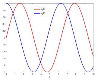
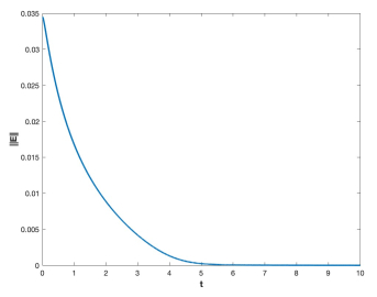
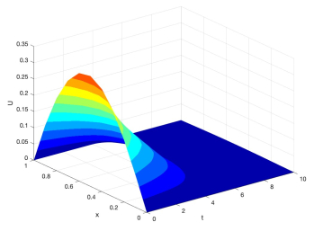
We establish an exponential stability result for a wave equation that includes weighted coefficients of structural damping and a delayed term. This study reveals cases where the delayed term may not be dominated by the damping term, yet the system is exponentially stable. Our coefficients do not obey necessarily the conditions that are usually imposed in the literature.
- wave equation,
- energy decay,
- time delay,
- strong damping,
- exponential stability
Citation: Waled Al-Khulaifi, Manal Alotibi, Nasser-Eddine Tatar. Exponential decay in a delayed wave equation with variable coefficients[J]. AIMS Mathematics, 2024, 9(10): 27770-27783. doi: 10.3934/math.20241348

Related Papers:

Abstract

We establish an exponential stability result for a wave equation that includes weighted coefficients of structural damping and a delayed term. This study reveals cases where the delayed term may not be dominated by the damping term, yet the system is exponentially stable. Our coefficients do not obey necessarily the conditions that are usually imposed in the literature.

References

[1]	S. Kim, D. Kim, Analytical modeling of thermoacoustic instability influences in gas turbine combustors: A detailed parameter sensitivity analysis, Case Stud. Therm. Eng., 59 (2024), 104595. http://dx.doi.org/10.1016/j.csite.2024.104595 doi: 10.1016/j.csite.2024.104595
[2]	J. Gibbons, D. Howard, A. Tyrrell, FPGA implementation of 1D wave equation for real-time audio synthesis, IEE P.-Comput. Dig. T., 152 (2005), 619–631. https://doi.org/10.1049/ip-cdt:20045178 doi: 10.1049/ip-cdt:20045178
[3]	Y. Chen, K. Ma, C. Ren, Y. Nan, P. Zhou, Mechanism of time-delay feedback control of suspension damping with an annular vibration-absorbing structure, J. Vibroeng., 25 (2023), 1561–1582. https://doi.org/10.21595/jve.2023.23291 doi: 10.21595/jve.2023.23291
[4]	A. Polyanin, V. Sorokin, A. Zhurov, Delay ordinary and partial differential equations, Chapman and Hall/CRC, 1 (2023). http://dx.doi.org/10.1201/9781003042310
[5]	T. Erneux, Applied delay differential equations, Springer eBook, 2009. http://dx.doi.org/10.1007/978-0-387-74372-1
[6]	V. Kolmanovskii, A. Myshkis, Introduction to the theory and applications of functional differential equations, Springer Science & Business Media, 2013.
[7]	G. Chen, Control and stabilization for the wave equation in a bounded domain, SIAM J. Control Optim., 17 (1979), 66–81. http://dx.doi.org/10.1137/0317007 doi: 10.1137/0317007
[8]	G. Chen, Control and stabilization for the wave Equation in a bounded domain, part Ⅱ, SIAM J. Control Optim., 19 (1981), 114–122. http://dx.doi.org/10.1137/0319009 doi: 10.1137/0319009
[9]	V. Komornik, Exact controllability and stabilization: The multiplier method, Elsevier Masson, 1994.
[10]	R. Datko, Representation of solutions and stability of linear differential-difference equations in a Banach space, J. Differ. Equations, 29 (1978), 105–166. http://dx.doi.org/10.1016/0022-0396(78)90043-8 doi: 10.1016/0022-0396(78)90043-8
[11]	R. Datko, J. Lagnese, M. Polis, An example on the effect of time delays in boundary feedback stabilization of wave equations, SIAM J. Control Optim., 24 (1986), 152–156. http://dx.doi.org/10.1137/0324007 doi: 10.1137/0324007
[12]	G. Xu, S. Yung, L. Li, Stabilization of wave systems with input delay in the boundary control, ESAIM Contr. Optim. Ca., 12 (2006), 770–785. http://dx.doi.org/10.1051/cocv:2006021 doi: 10.1051/cocv:2006021
[13]	S. Nicaise, C. Pignotti, Stability and instability results of the wave equation with a delay term in the boundary or internal feedbacks, SIAM J. Control Optim., 45 (2006), 1561–1585. http://dx.doi.org/10.1016/j.jmaa.2004.01.048 doi: 10.1016/j.jmaa.2004.01.048
[14]	S. Nicaise, C. Pignotti, Exponential stability of abstract evolution equations with time delay, J. Evol. Equ., 15 (2015), 107–129. http://dx.doi.org/10.1007/s00028-014-0251-5 doi: 10.1007/s00028-014-0251-5
[15]	M. Kirane, B. Said-Houari, Existence and asymptotic stability of a viscoelastic wave equation with a delay, Z. Angew. Math. Phys., 62 (2011), 1065–1082. http://dx.doi.org/10.1007/s00033-011-0145-0 doi: 10.1007/s00033-011-0145-0
[16]	F. Alabau-Boussouira, S. Nicaise, C. Pignotti, Exponential stability of the wave equation with memory and time delay, In: New prospects in direct, inverse and control problems for evolution equations, Springer Indam Series, 10 (2014), 1–22. http://dx.doi.org/10.1007/978-3-319-11406-4-1
[17]	A. Guesmia, Well-posedness and exponential stability of an abstract evolution equation with infinite memory and time delay, IMA J. Math. Control I., 30 (2013), 507–526. http://dx.doi.org/10.1093/imamci/dns039 doi: 10.1093/imamci/dns039
[18]	S. Park, Global existence, energy decay and blow-up of solutions for wave equations with time delay and logarithmic source, Adv. Differ. Equ., 2020 (2020), 631. http://dx.doi.org/10.1186/s13662-020-03037-6 doi: 10.1186/s13662-020-03037-6
[19]	G. Liu, H. Yue, H. Zhang, Long time behavior for a wave equation with time delay, Taiwan. J. Math., 21 (2017), 107–129. Available from: https://www.jstor.org/stable/90000350.
[20]	S. Wu, Asymptotic behavior for a viscoelastic wave equation with a delay term, Taiwan. J. Math., 17 (2013), 765–784. http://dx.doi.org/10.11650/tjm.17.2013.2517 doi: 10.11650/tjm.17.2013.2517
[21]	A. Benaissa, S. Messaoudi, Global existence and energy decay of solutions for a nondissipative wave equation with a time-varying delay term, Springer International Publishing, 2013. Available from: http://dx.doi.org/10.1007/978-3-319-00125-8_1.
[22]	H. Yüksekkaya, E. Pișkin, S. Boulaaras, B. Cherif, S. Zubair, Existence, nonexistence, and stability of solutions for a delayed plate equation with the logarithmic source, Adv. Math. Phys., 2021 (2021), 1–11. http://dx.doi.org/10.1155/2021/8561626 doi: 10.1155/2021/8561626
[23]	Z. Yang, Existence and energy decay of solutions for the Euler-Bernoulli viscoelastic equation with a delay, Z. Angew. Math. Phys., 66 (2015), 727–745. http://dx.doi.org/10.1007/s00033-014-0429-2 doi: 10.1007/s00033-014-0429-2
[24]	M. Mustafa, M. Kafini, Decay rates for memory-type plate system with delay and source term, Math. Meth. Appl. S., 40 (2017), 883–895. http://dx.doi.org/10.1002/mma.4015 doi: 10.1002/mma.4015
[25]	A. Benaissa, S. Messaoudi, A. Benguessoum, Energy decay of solutions for a wave equation with a constant weak delay and a weak internal feedback, Electron. J. Qual. Theo., 2014, 1–13. http://dx.doi.org/10.14232/ejqtde.2014.1.11
[26]	V. Barros, C. Nonato, C. Raposo, Global existence and energy decay of solutions for a wave equation with non-constant delay and nonlinear weights, Electron. Res. Arch., 28 (2020), 205–220. http://dx.doi.org/10.3934/era.2020014 doi: 10.3934/era.2020014
[27]	Q. Dai, Z. Yang, Global existence and exponential decay of the solution for a viscoelastic wave equation with a delay, Z. Angew. Math. Phys., 65 (2014), 885–903. http://dx.doi.org/10.1007/s00033-013-0365-6 doi: 10.1007/s00033-013-0365-6
[28]	S. Messaoudi, A. Fareh, N. Doudi, Well posedness and exponential stability in a wave equation with a strong damping and a strong delay, J. Math. Phys., 57 (2016), 111501. http://dx.doi.org/10.1063/1.4966551 doi: 10.1063/1.4966551
[29]	H. Makheloufi, M. Bahlil, Global well-posedness and stability results for an abstract viscoelastic equation with a non-constant delay term and nonlinear weight, Ric. Mat., 73 (2021), 433–469. http://dx.doi.org/10.1007/s11587-021-00617-w doi: 10.1007/s11587-021-00617-w
[30]	B. Feng, General decay for a viscoelastic wave equation with strong time-dependent delay, Bound. Value Probl., 2017. http://dx.doi.org/10.1186/s13661-017-0789-6
[31]	C. Enyi, S. Mukiawa, Decay estimate for a viscoelastic plate equation with strong time-varying delay, Ann. U. Ferrara, 66 (2020), 339–357. http://dx.doi.org/10.1007/s11565-020-00346-2 doi: 10.1007/s11565-020-00346-2
[32]	W. Al-Khulaifi, T. Diagana, A. Guesmia, Well-posedness and stability results for some nonautonomous abstract linear hyperbolic equations with memory, Semigroup Forum, 105 (2022), 351–373. https://doi.org/10.1007/s00233-022-10284-4 doi: 10.1007/s00233-022-10284-4
[33]	N. Tatar, Stability for the damped wave equation with neutral delay, Math. Nachr., 290 (2017), 2401–2412. http://dx.doi.org/10.1002/mana.201600229 doi: 10.1002/mana.201600229
[34]	T. Wang, Inequalities and stability for a linear scalar functional differential equation, J. Math. Anal. Appl., 298 (2004), 33–44. http://dx.doi.org/10.1016/j.jmaa.2004.01.048 doi: 10.1016/j.jmaa.2004.01.048

Reader Comments

Your name:*

Email:*
© 2024 the Author(s), licensee AIMS Press. This is an open access article distributed under the terms of the Creative Commons Attribution License (http://creativecommons.org/licenses/by/4.0)