A Bhattacharyya Triangular intuitionistic fuzzy sets with a Owa operator-based decision making for optimal portfolio selection in Saudi exchange

Sunil Kumar Sharma; Sunil Kumar Sharma

doi:10.3934/math.20241324

AIMS Mathematics

2024, Volume 9, Issue 10: 27247-27271. doi: 10.3934/math.20241324

Previous Article Next Article

Research article

A Bhattacharyya Triangular intuitionistic fuzzy sets with a Owa operator-based decision making for optimal portfolio selection in Saudi exchange

Sunil Kumar Sharma ^,

Department of Information System, College of Computer and Information Sciences, Majmaah University, Majmaah 11952, Saudi Arabia

Received: 22 June 2024 Revised: 16 August 2024 Accepted: 22 August 2024 Published: 20 September 2024
MSC : 03E72, 62C86

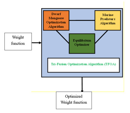
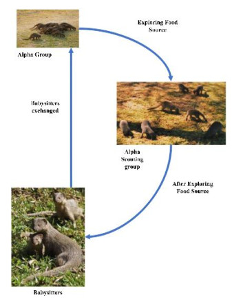
The capital market in Saudi Arabia is fast growing. Assurance of an informed decision while investing in the Saudi Stock Exchange is critical. There has also been an increased quest for advanced decision-making tools due to complexities in selecting a given portfolio, which remains a critical issue of concern among investors in the face of modern investment environment challenges. The research paper offered shall deliver an innovative MCDM technique through which an MCDM model shall be developed in the Saudi Stock Exchange. This MCDM model uses BTIFS with an OWA operator. A novelty of the proposed study is identifying the optimal weight that will be obtained through a newly developed optimization technique known as TFOA. TFOA is a hybrid methodology that brings on board the strengths of DMOA, MPA, and EO for a more precise and efficient calculation of the ideal weights in the portfolio selection process. This would improve the adaptability and effectiveness of the suggested MCDM structure. The effectiveness of the approach is established by comparative analysis with the already existing methods of MCDM, which proves it superior for the optimization of investment portfolios. Sensitivity analysis also conducted to evaluate the strength and dependability of the suggested method. The ranking of weighted portfolios by the ELECTRE method is also, which more establishes the applicability of BTIFS-OWA in real life. The results indicate that the BTIFS-OWA approach along with the TFOA for determining optimal weights provides significant improvements in decision-making accuracy and portfolio optimization compared to traditional methods.
- multiple Criteria decision-making,
- Bhattacharyya distance,
- Triangular intuitionistic fuzzy sets,
- OWA operator,
- Saudi stock market
Citation: Sunil Kumar Sharma. A Bhattacharyya Triangular intuitionistic fuzzy sets with a Owa operator-based decision making for optimal portfolio selection in Saudi exchange[J]. AIMS Mathematics, 2024, 9(10): 27247-27271. doi: 10.3934/math.20241324

Related Papers:

Abstract

The capital market in Saudi Arabia is fast growing. Assurance of an informed decision while investing in the Saudi Stock Exchange is critical. There has also been an increased quest for advanced decision-making tools due to complexities in selecting a given portfolio, which remains a critical issue of concern among investors in the face of modern investment environment challenges. The research paper offered shall deliver an innovative MCDM technique through which an MCDM model shall be developed in the Saudi Stock Exchange. This MCDM model uses BTIFS with an OWA operator. A novelty of the proposed study is identifying the optimal weight that will be obtained through a newly developed optimization technique known as TFOA. TFOA is a hybrid methodology that brings on board the strengths of DMOA, MPA, and EO for a more precise and efficient calculation of the ideal weights in the portfolio selection process. This would improve the adaptability and effectiveness of the suggested MCDM structure. The effectiveness of the approach is established by comparative analysis with the already existing methods of MCDM, which proves it superior for the optimization of investment portfolios. Sensitivity analysis also conducted to evaluate the strength and dependability of the suggested method. The ranking of weighted portfolios by the ELECTRE method is also, which more establishes the applicability of BTIFS-OWA in real life. The results indicate that the BTIFS-OWA approach along with the TFOA for determining optimal weights provides significant improvements in decision-making accuracy and portfolio optimization compared to traditional methods.

References

[1]	A. Thakkar, K. Chaudhari, Fusion in stock market prediction: A decade survey on the necessity, recent developments, and potential future directions, Inform. Fusion, 65 (2021), 95–107. https://doi.org/10.1016/j.inffus.2020.08.019 doi: 10.1016/j.inffus.2020.08.019
[2]	G. Kumar, S. Jain, U. P. Singh, Stock market forecasting using computational intelligence: A survey, Arch. Computat. Methods Eng., 28 (2021), 1069–1101. https://doi.org/10.1007/s11831-020-09413-5 doi: 10.1007/s11831-020-09413-5
[3]	M. Abreu, V. Mendes, Do individual investors trade differently in different financial markets, The Eur. J. Financ., 26 (2020), 1253–1270. https://doi.org/10.1080/1351847X.2019.1709524 doi: 10.1080/1351847X.2019.1709524
[4]	J. F. Ma, J. D. Harstvedt, R. Jaradat, B. Smith, Sustainability driven multi-criteria project portfolio selection under uncertain decision-making environment, Comput. Ind. Eng., 140 (2020), 106236. https://doi.org/10.1016/j.cie.2019.106236 doi: 10.1016/j.cie.2019.106236
[5]	J. W. Goodell, S. Kumar, W. M. Lim, D. Pattnaik, Artificial intelligence and machine learning in finance: Identifying foundations, themes, and research clusters from bibliometric analysis, J. Behav. Exp. Financ., 32 (2021), 100577. https://doi.org/10.1016/j.jbef.2021.100577 doi: 10.1016/j.jbef.2021.100577
[6]	S. R. Das, D. Ostrov, A. Radhakrishnan, D. Srivastav, Dynamic portfolio allocation in goals-based wealth management, Comput. Manag. Sci., 17 (2020), 613–640. https://doi.org/10.1007/s10287-019-00351-7 doi: 10.1007/s10287-019-00351-7
[7]	M. R. Galankashi, F. M. Rafiei, M. Ghezelbash, Portfolio selection: A fuzzy-ANP approach, Financ. Innov., 6 (2020), 17. https://doi.org/10.1186/s40854-020-00175-4 doi: 10.1186/s40854-020-00175-4
[8]	H. Taherdoost, M. Madanchian, Multi-criteria decision making (MCDM) methods and concepts, Encyclopedia, 3 (2023), 77–87. https://doi.org/10.3390/encyclopedia3010006 doi: 10.3390/encyclopedia3010006
[9]	L. A. Zadeh, Fuzzy sets, Information and Control, 8 (1965), 338–353. https://doi.org/10.1016/S0019-9958(65)90241-X doi: 10.1016/S0019-9958(65)90241-X
[10]	K. T. Atanassov, Intuitionistic fuzzy sets, Fuzzy Set. Syst., 20 (1986), 87–96. https://doi.org/10.1016/S0165-0114(86)80034-3 doi: 10.1016/S0165-0114(86)80034-3
[11]	11I. Despi, D. Opris, E. Yalcin, Generalised Atanassov intuitionistic fuzzy sets, The Fifth International Conference on Information, Process, and Knowledge Management, France, 2013, 51–56.
[12]	S. Perçin, Circular supplier selection using interval-valued intuitionistic fuzzy sets, Environ. Dev. Sustain., 24 (2022), 5551–5581. https://doi.org/10.1007/s10668-021-01671-y doi: 10.1007/s10668-021-01671-y
[13]	S. N. M. Kodukulla, V. Sireesha, A novel ranking approach to rank interval-valued trapezoidal intuitionistic fuzzy sets by using the concept of centroids, SN Comput. Sci., 5 (2024), 493. https://doi.org/10.1007/s42979-024-02861-x doi: 10.1007/s42979-024-02861-x
[14]	S. N. M. Kodukulla, V. Sireesha, An extended VIKOR method for interval-valued trapezoidal intuitionistic fuzzy decision making, Mathematical Statistician and Engineering Applications, 71 (2022), 4390–4403. https://doi.org/10.17762/msea.v71i4.1025 doi: 10.17762/msea.v71i4.1025
[15]	I. Singuluri, N. R. Shankar, A contemporary transportation perspective for determination of type–1 triangular intuitionistic fuzzy transportation problem, Turk. J. Physiother. R., 32 (2021), 7157–7163.
[16]	M. Qiyas, S. Abdullah, Y. Liu, M. Naeem, Multi-criteria decision support systems based on linguistic intuitionistic cubic fuzzy aggregation operators, J. Ambient Intell. Human. Comput., 12 (2021), 8285–8303. https://doi.org/10.1007/s12652-020-02563-1 doi: 10.1007/s12652-020-02563-1
[17]	M. H. Alamoudi, O. A. Bafail, BWM—RAPS approach for evaluating and ranking banking sector companies based on their financial indicators in the Saudi stock market, J. Risk Financial Manag., 15 (2022), 467. https://doi.org/10.3390/jrfm15100467 doi: 10.3390/jrfm15100467
[18]	V. L. G. Nayagam, J. Murugan, Triangular approximation of intuitionistic fuzzy numbers on multi-criteria decision making problem, Soft Comput., 25 (2021), 9887–9914. https://doi.org/10.1007/s00500-020-05346-0 doi: 10.1007/s00500-020-05346-0
[19]	H. Hashemi, P. Ghoddousi, F. Nasirzadeh, Sustainability indicator selection by a novel triangular intuitionistic fuzzy decision-making approach in highway construction projects, Sustainability, 13 (2021), 1477. https://doi.org/10.3390/su13031477 doi: 10.3390/su13031477
[20]	F. D. Remadi, H. M. Frikha, The triangular intuitionistic fuzzy extension of the CODAS method for solving multi-criteria group decision making, 2020 International Multi-Conference on: "Organization of Knowledge and Advanced Technologies", Tunis, Tunisia, 2020, 1–6. https://doi.org/10.1109/OCTA49274.2020.9151786
[21]	F. D. Remadi, H. M. Frikha, The triangular intuitionistic fuzzy numbers CODAS method for solving green material selection problem, International Journal of Operational Research, 46 (2023), 398–415. https://doi.org/10.1504/IJOR.2023.129409 doi: 10.1504/IJOR.2023.129409
[22]	M. Saeed, A. Mehmood, A. Anwar, An extension of TOPSIS based on linguistic terms in triangular intuitionistic fuzzy structure, Punjab Univ. J. Math., 53 (2021), 409–424. https://doi.org/10.52280/pujm.2021.530604 doi: 10.52280/pujm.2021.530604
[23]	A. Prakash, M. Suresh, Ranking triangular intuitionistic fuzzy numbers: A nagel point approach and applications in multi-criteria decision making, in press. https://doi.org/10.21203/rs.3.rs-3897760/v1
[24]	O. M. Babatunde, J. L. Munda, Y. Hamam, Triangular intuitionistic fuzzy aggregating and ranking function approach for the rating of battery 'End-of-Life' handling alternatives, Energies, 15 (2022), 2248. https://doi.org/10.3390/en15062248 doi: 10.3390/en15062248
[25]	X. L. Geng, Y. Ma, N-Intuitionistic polygonal fuzzy aggregation operators and their application to multi-attribute decision making, IEEE Access, 8 (2020), 162903–162916. https://doi.org/10.1109/ACCESS.2020.3018957 doi: 10.1109/ACCESS.2020.3018957
[26]	S. S. Biswas, B. Alam, M. N. Doja, An algorithm for extracting intuitionistic fuzzy shortest path in a graph, Appl. Comput. Intell. S., 2013 (2013), 970197. https://doi.org/10.1155/2013/970197 doi: 10.1155/2013/970197
[27]	K. Bisht, A. Kumar, Stock portfolio selection hybridizing fuzzy base-criterion method and evidence theory in triangular fuzzy environment, Oper. Res. Forum, 3 (2022), 53. https://doi.org/10.1007/s43069-022-00167-3 doi: 10.1007/s43069-022-00167-3
[28]	H. B. Jiang, B. Q. Hu, A decision-theoretic fuzzy rough set in hesitant fuzzy information systems and its application in multi-attribute decision-making, Inform. Sci., 579 (2021), 103–127. https://doi.org/10.1016/j.ins.2021.07.094 doi: 10.1016/j.ins.2021.07.094
[29]	J. D. Zhou, X. Li, Multi-period mean-semi-entropy portfolio management with transaction costs and bankruptcy control, J. Ambient Intell. Human. Comput., 12 (2021), 705–715. https://doi.org/10.1007/s12652-020-02053-4 doi: 10.1007/s12652-020-02053-4
[30]	M. Narang, M. C. Joshi, K. Bisht, A. Pal, Stock portfolio selection using a new decision-making approach based on the integration of fuzzy CoCoSo with Heronian mean operator, Decision Making: Applications in Management and Engineering, 5 (2022), 90–112. https://doi.org/10.31181/dmame0310022022n doi: 10.31181/dmame0310022022n
[31]	M. Jagtap, P. Karande, The m-polar fuzzy set ELECTRE-I with revised Simos' and AHP weight calculation methods for selection of non-traditional machining processes, Decision Making: Applications in Management and Engineering, 6 (2023), 240–281. https://doi.org/10.31181/dmame060129022023j doi: 10.31181/dmame060129022023j
[32]	A. R. Mishra, P. Rani, F. Cavallaro, A. F. Alrasheedi, Assessment of sustainable wastewater treatment technologies using interval-valued intuitionistic fuzzy distance measure-based MAIRCA method, Facta Univ.-Ser. Mech., 21 (2023), 359–386. https://doi.org/10.22190/FUME230901034M doi: 10.22190/FUME230901034M
[33]	R. Isabels, A. F. Vinodhini, A. Viswanathan, Evaluating and ranking metaverse platforms using intuitionistic trapezoidal fuzzy VIKOR MCDM: Incorporating score and accuracy functions for comprehensive assessment, Decision Making: Applications in Management and Engineering, 7 (2024), 54–78. https://doi.org/10.31181/dmame712024858 doi: 10.31181/dmame712024858
[34]	P. Wang, B. Y. Zhu, Y. Yu, Z. Ali, B. Almohsen, Complex intuitionistic fuzzy DOMBI prioritized aggregation operators and their application for resilient green supplier selection, Facta Univ.-Ser. Mech., 21 (2023), 339–357. https://doi.org/10.22190/FUME230805029W doi: 10.22190/FUME230805029W
[35]	S. Sharma, S. Chandra, K. A. Singh, Total productive maintenance using cosine maximization multi attribute method, Ad Alta Interdiscip., 2020 (2020), 110–117.
[36]	J. X. Tang, J. D. Cheng, D. L. Xiang, C. B. Hu, Large-difference-scale target detection using a revised Bhattacharyya distance in SAR images, IEEE Geosci. Remote S., 19 (2022), 4506205. https://doi.org/10.1109/LGRS.2022.3161931 doi: 10.1109/LGRS.2022.3161931
[37]	P. F. Zhang, D. X. Wang, Z. Yu, Y. J. Zhang, T. Jiang, T. R. Li, A multi-scale information fusion-based multiple correlations for unsupervised attribute selection, Inform. Fusion, 106 (2024), 102276. https://doi.org/10.1016/j.inffus.2024.102276 doi: 10.1016/j.inffus.2024.102276
[38]	P. F. Zhang, T. R. Li, Z. Yuan, Z. X. Deng, G. Q. Wang, D. X. Wang, et al., A possibilistic information fusion-based unsupervised feature selection method using information quality measures, IEEE T. Fuzzy Syst., 31 (2023), 2975–2988. https://doi.org/10.1109/TFUZZ.2023.3238803 doi: 10.1109/TFUZZ.2023.3238803
[39]	K. Bhattacharya, S. K. De, Decision making under intuitionistic fuzzy metric distances, Annals of Optimization Theory and Practice, 3 (2020), 49–64. https://doi.org/10.22121/aotp.2020.250749.1043 doi: 10.22121/aotp.2020.250749.1043
[40]	A. Bhattacharya, M. Pal, Fuzzy covering problem of fuzzy graphs and its application to investigate the Indian economy in new normal, J. Appl. Math. Comput., 68 (2022), 479–510. https://doi.org/10.1007/s12190-021-01539-4 doi: 10.1007/s12190-021-01539-4
[41]	S. F. Bi, M. Broggi, M. Beer, The role of the Bhattacharyya distance in stochastic model updating, Mech. Syst. Signal Pr., 117 (2019), 437–452. https://doi.org/10.1016/j.ymssp.2018.08.017 doi: 10.1016/j.ymssp.2018.08.017
[42]	F. J. Aherne, N. A. Thacker, P. I. Rockett, The Bhattacharyya metric as an absolute similarity measure for frequency coded data, Kybernetika, 34 (1998), 363–368.

Reader Comments

Your name:*

Email:*
© 2024 the Author(s), licensee AIMS Press. This is an open access article distributed under the terms of the Creative Commons Attribution License (http://creativecommons.org/licenses/by/4.0)