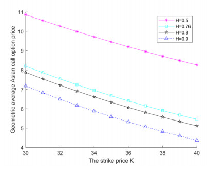
Considering the characteristics of long-range correlations in financial markets, the issue of valuing geometric average Asian options is examined, assuming that the variations of the underlying asset follow the mixed sub-fractional Brownian motion, and the dynamics of short-term interest rate satisfies the mixed sub-fractional Vasicek model. Based on the principle of no arbitrage, the definite solution of PDE of a zero-coupon bond for geometric average Asian options under the circumstance of the mixed sub-fractional is given by the delta hedging technique. The derivation of the explicit pricing formula for geometric average Asian options with fixed strike price is achieved through the utilization of multiple variable substitutions. Furthermore, we perform numerical calculations to analyze the performance of the model.
Citation: Xinyi Wang, Chunyu Wang. Pricing geometric average Asian options in the mixed sub-fractional Brownian motion environment with Vasicek interest rate model[J]. AIMS Mathematics, 2024, 9(10): 26579-26601. doi: 10.3934/math.20241293
Considering the characteristics of long-range correlations in financial markets, the issue of valuing geometric average Asian options is examined, assuming that the variations of the underlying asset follow the mixed sub-fractional Brownian motion, and the dynamics of short-term interest rate satisfies the mixed sub-fractional Vasicek model. Based on the principle of no arbitrage, the definite solution of PDE of a zero-coupon bond for geometric average Asian options under the circumstance of the mixed sub-fractional is given by the delta hedging technique. The derivation of the explicit pricing formula for geometric average Asian options with fixed strike price is achieved through the utilization of multiple variable substitutions. Furthermore, we perform numerical calculations to analyze the performance of the model.

| [1] | F. Black, M. Scholes, The pricing of options and corporate liabilities, J. Polit. Econ., 81 (1973), 637–654. |
| [2] |
K. Reddy, V. Clinton, Simulating stock prices using geometric Brownian motion: evidence from Australian companies, Australas. Account. Bu., 10 (2016), 23–47. https://doi.org/10.14453/aabfj.v10i3.3 doi: 10.14453/aabfj.v10i3.3

|
| [3] |
K. Suganthi, G. Jayalalitha, Geometric Brownian motion in stock prices, J. Phys. Conf. Ser., 1377 (2019), 012016. https://doi.org/10.1088/1742-6596/1377/1/012016 doi: 10.1088/1742-6596/1377/1/012016
|
| [4] |
B. B. Mandelbrot, J. W. Van Ness, Fractional Brownian motions, fractional noises and applications, SIAM Rev., 10 (1968), 422–437. https://doi.org/10.1137/1010093 doi: 10.1137/1010093
|
| [5] |
L. C. G. Rogers, Arbitrage with fractional Brownian motion, Math. Financ., 7 (1997), 95–105. https://doi.org/10.1111/1467-9965.00025 doi: 10.1111/1467-9965.00025
|
| [6] |
P. Cheridito, Arbitrage in fractional Brownian motion models, Finance Stochast, 7 (2003), 533–553. https://doi.org/10.1007/s007800300101 doi: 10.1007/s007800300101
|
| [7] |
T. Bojdecki, L. G. Gorostiza, A. Talarczyk, Sub-fractional Brownian motion and its relation to occupation times, Stat. Probabil. Lett., 69 (2004), 405–419. https://doi.org/10.1016/j.spl.2004.06.035 doi: 10.1016/j.spl.2004.06.035
|
| [8] |
C. Tubor, Some properties of the sub-fractional Brownian motion, Stochastics, 79 (2007), 431–448. https://doi.org/10.1080/17442500601100331 doi: 10.1080/17442500601100331
|
| [9] |
F. Xu, R. Li, The pricing formulas of compound option based on the sub-fractional Brownian motion model, J. Phys.: Conf. Ser., 1053 (2018), 012027. https://doi.org/10.1088/1742-6596/1053/1/012027 doi: 10.1088/1742-6596/1053/1/012027
|
| [10] |
Z. Guo, Y. Liu, L. Dai, European option pricing under sub-fractional Brownian motion regime in discrete time, Fractal Fract., 8 (2023), 13. https://doi.org/10.3390/fractalfract8010013 doi: 10.3390/fractalfract8010013
|
| [11] |
X. Wang, Z. Yang, P. Cao, S. Wang, The closed-form option pricing formulas under the sub-fractional Poisson volatility models, Chaos Solitons Fract., 148 (2021), 111012. https://doi.org/10.1016/j.chaos.2021.111012 doi: 10.1016/j.chaos.2021.111012
|
| [12] |
H. Jafari, H. Farahani, An approximate approach to fuzzy stochastic differential equations under sub-fractional Brownian motion, Stoch. Dynam., 23 (2023), 2350017. https://doi.org/10.1142/S021949372350017X doi: 10.1142/S021949372350017X
|
| [13] |
X. Zhang, W. Xiao, Arbitrage with fractional Gaussian processes, Phys. A, 471 (2017), 620–628. https://doi.org/10.1016/j.physa.2016.12.064 doi: 10.1016/j.physa.2016.12.064
|
| [14] |
C. EI-Nouty, M. Zili, On the sub-mixed fractional Brownian motion, Appl. Math. J. Chin. Univ., 30 (2015), 27–43. https://doi.org/10.1007/s11766-015-3198-6 doi: 10.1007/s11766-015-3198-6
|
| [15] |
A. A. Araneda, N. Bertschinger, The sub-fractional CEV model, Phys. A, 573 (2021), 125974. https://doi.org/10.1016/J.PHYSA.2021.125974 doi: 10.1016/J.PHYSA.2021.125974
|
| [16] |
C. Bender, T. Sottinen, E. Valkeila, Pricing by hedging and no-arbitrage beyond semimartingales, Finance Stoch., 12 (2008), 441–468. https://doi.org/10.1007/s00780-008-0074-8 doi: 10.1007/s00780-008-0074-8
|
| [17] |
J. Guo, W. Kang, Y. Wang, Option pricing under sub-mixed fractional Brownian motion based on time-varying implied volatility using intelligent algorithms, Soft Comput., 27 (2023), 15225–15246. https://doi.org/10.1007/s00500-023-08647-2 doi: 10.1007/s00500-023-08647-2
|
| [18] |
C. Cai, Q. Wang, W. Xiao, Mixed sub-fractional Brownian motion and drift estimation of related Ornstein-Uhlenbeck process, Commun. Math. Stat., 11 (2023), 229–255. https://doi.org/10.1007/s40304-021-00245-8 doi: 10.1007/s40304-021-00245-8
|
| [19] |
O. Vasicek, An equilibrium characterization of the term structure, J. Financ. Econ., 5 (1977), 177–188. https://doi.org/10.1016/0304-405X(77)90016-2 doi: 10.1016/0304-405X(77)90016-2
|
| [20] |
C. O. Ewald, Y. Wu, A. Zhang, Pricing Asian options with stochastic convenience yield and jumps, Quant. Financ., 23 (2023), 677–692. https://doi.org/10.1080/14697688.2022.2160799 doi: 10.1080/14697688.2022.2160799
|
| [21] |
Y. Yun, L. Gao, Pricing and analysis of European chooser option under the Vasicek interest rate mode, Int. J. Theor. Appl. Math., 6 (2020), 19–27. https://doi.org/10.11648/j.ijtam.20200602.11 doi: 10.11648/j.ijtam.20200602.11
|
| [22] |
Y. Fu, S. Zhou, X. Li, F. Rao, Multi-assets Asian rainbow options pricing with stochastic interest rates obeying the Vasicek model, AIMS Math., 8 (2023), 10685–10710. https://doi.org/10.3934/math.2023542 doi: 10.3934/math.2023542
|
| [23] |
W. Xiao, W. Zhang, X. Zhang, X. Chen, The valuation of equity warrants under the fractional Vasicek process of the short-term interest rate, Phys. A, 394 (2014), 320–337. https://doi.org/10.1016/j.physa.2013.09.033 doi: 10.1016/j.physa.2013.09.033
|
| [24] |
Y. Han, N. Li, Calibrating fractional Vasicek model, Commun. Stat., 52 (2023), 4429–4443. https://doi.org/10.1080/03610926.2021.1994609 doi: 10.1080/03610926.2021.1994609
|
| [25] |
P. C. Lukman, B. D. Handari, H. Tasman, Study on European put option pricing with underlying asset zero-coupon bond and interest rate following the Vasicek model with jump, J. Phys.: Conf. Ser., 1725 (2021), 012092. https://doi.org/10.1088/1742-6596/1725/1/012092 doi: 10.1088/1742-6596/1725/1/012092
|
| [26] |
Z. Guo, X. Wang, Y. Zhang, Option pricing of geometric Asian options in a subdiffusive Brownian motion regime, AIMS Math., 5 (2020), 5332–5343. https://doi.org/10.3934/math.2020342 doi: 10.3934/math.2020342
|
| [27] | B. B. Mandelbrot, Statistical methodology for nonperiodic cycles: from the covariance to R/S analysis, Ann. Econ. Soc. Meas., 1 (1972), 259–290. |


Figures(5) / Tables(3)

Xinyi Wang, Chunyu Wang. Pricing geometric average Asian options in the mixed sub-fractional Brownian motion environment with Vasicek interest rate model[J]. AIMS Mathematics, 2024, 9(10): 26579-26601. doi: 10.3934/math.20241293


 DownLoad: