Mathematical models, especially complex nonlinear systems, are always difficult to analyze and synthesize, and researchers need effective and suitable control methods to address these issues. In the present work, we proposed a hybrid method that combines the well-known Takagi-Sugeno fuzzy model with wavelet decomposition to investigate nonlinear systems characterized by the presence of mixed nonlinearities. Here, one nonlinearity is super-linear and convex, and other is sub-linear, concave, and singular at zero, which leads to difficulties in the analysis, as is known in PDE theory. Linear and polynomial fuzzy models were combined with wavelets to ensure an improvement in both methods for investigating such problems. The results showed a high performance compared with existing methods via error estimates and Lyapunov theory of stability. The model was applied to a prototype nonlinear Schrödinger dynamical system.
Citation: Anouar Ben Mabrouk, Abdulaziz Alanazi, Zaid Bassfar, Dalal Alanazi. New hybrid model for nonlinear systems via Takagi-Sugeno fuzzy approach[J]. AIMS Mathematics, 2024, 9(9): 23197-23220. doi: 10.3934/math.20241128
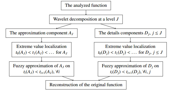
Mathematical models, especially complex nonlinear systems, are always difficult to analyze and synthesize, and researchers need effective and suitable control methods to address these issues. In the present work, we proposed a hybrid method that combines the well-known Takagi-Sugeno fuzzy model with wavelet decomposition to investigate nonlinear systems characterized by the presence of mixed nonlinearities. Here, one nonlinearity is super-linear and convex, and other is sub-linear, concave, and singular at zero, which leads to difficulties in the analysis, as is known in PDE theory. Linear and polynomial fuzzy models were combined with wavelets to ensure an improvement in both methods for investigating such problems. The results showed a high performance compared with existing methods via error estimates and Lyapunov theory of stability. The model was applied to a prototype nonlinear Schrödinger dynamical system.

| [1] |
M. S. Aslam, H. Bilal, S. S. Band, P. Ghasemi, Modeling of nonlinear supply chain management with lead-times based on Takagi-Sugeno fuzzy control model, Eng. Appl. Artif. Intell., 133 (2024), 108131. https://doi.org/10.1016/j.engappai.2024.108131 doi: 10.1016/j.engappai.2024.108131

|
| [2] | S. Arfaoui, A. Ben Mabrouk, C. Cattani, Wavelet analysis: basic concepts and applications, New York: Chapman and Hall/CRC, 2021. https://doi.org/10.1201/9781003096924 |
| [3] |
S. A. Ahmadi, P. Ghasemi, Pricing strategies for online hotel searching: a fuzzy inference system procedure, Kybernetes, 52 (2023), 4913–4936. https://doi.org/10.1108/K-03-2022-0427 doi: 10.1108/K-03-2022-0427
|
| [4] |
D. Aleksovski, J. Kocijan, S. Dzeroski, Ensembles of fuzzy linear model trees for the identification of multioutput systems, IEEE Trans. Fuzzy Syst., 24 (2016), 916–929. https://doi.org/10.1109/TFUZZ.2015.2489234 doi: 10.1109/TFUZZ.2015.2489234
|
| [5] |
J. Awrejcewicz, V. A. Krysko, I. V. Papkova, T. V. Yakovleva, N. A. Zagniboroda, M. V. Zhigalov, et al., Application of the Lyapunov exponents and wavelets to study and control of plates and shells, Comput. Numer. Simul., 2014. https://doi.org/10.5772/57452 doi: 10.5772/57452
|
| [6] |
J. Awrejcewicz, A. V. Krysko, V. Soldatov, On the wavelet transform application to a study of chaotic vibrations of the infinite length flexible panels driven longitudinally, Int. J. Bifur. Chaos, 19 (2009), 3347–3371. https://doi.org/10.1142/S0218127409024803 doi: 10.1142/S0218127409024803
|
| [7] |
J. J. Buckley, Universal fuzzy controllers, Automatica, 28 (1992), 1245–1248. https://doi.org/10.1016/0005-1098(92)90068-Q doi: 10.1016/0005-1098(92)90068-Q
|
| [8] | A. Ben Mabrouk, M. L. Ben Mohamed, On some critical and slightly super-critical sub-superlinear equations, Far East J. Appl. Math., 23 (2006), 73–90. |
| [9] |
A. Ben Mabrouk, M. L. Ben Mohamed, Nodal solutions for some nonlinear elliptic equations, Appl. Math. Comput., 186 (2007), 589–597. https://doi.org/10.1016/j.amc.2006.08.003 doi: 10.1016/j.amc.2006.08.003
|
| [10] |
A. Ben Mabrouk, M. L. Ben Mohamed, Phase plane analysis and classification of solutions of a mixed sublinear-superlinear elliptic problem, Nonlinear Anal., 70 (2009), 1–15. https://doi.org/10.1016/j.na.2007.11.041 doi: 10.1016/j.na.2007.11.041
|
| [11] |
R. Bentez, V. J. Bolos, M. E. Ramrez, A wavelet-based tool for studying non-periodicity, Comput. Math. Appl., 60 (2010), 634–641. https://doi.org/10.1016/j.camwa.2010.05.010 doi: 10.1016/j.camwa.2010.05.010
|
| [12] |
A. Bakdi, A. Hentout, H. Boutami, A. Maoudj, O. Hachour, B. Bouzouia, Optimal path planning and execution for mobile robots using genetic algorithm and adaptive fuzzy-logic control, Robot. Autonomous Syst., 89 (2017), 95–109. https://doi.org/10.1016/j.robot.2016.12.008 doi: 10.1016/j.robot.2016.12.008
|
| [13] |
A. Ben Mabrouk, O. Zaafrane, Wavelet fuzzy hybrid model for physico-financial signals, J. Appl. Statist., 40 (2013), 1453–1463. https://doi.org/10.1080/02664763.2013.786690 doi: 10.1080/02664763.2013.786690
|
| [14] |
R. Chteoui, A. F. Aljohani, A. Ben Mabrouk, Classification and simulation of chaotic behavior of the solutions of a mixed nonlinear Schrodinger system, Electron. Res. Arch., 29 (2021), 2561–2597. https://doi.org/10.3934/era.2021002 doi: 10.3934/era.2021002
|
| [15] | R. Chteoui, A. Ben Mabrouk, C. Cattani, Mixed concave-convex sub-superlinear Schrodinger equation: survey and development of some new cases, In: Nonlinear analysis and global optimization, Cham: Springer, 2021,109–162. https://doi.org/10.1007/978-3-030-61732-5_5 |
| [16] | F. Chevrie, F. Guely, La logique floue, Cah. Tech., 191 (1998), 1–28. |
| [17] |
J. Cozar, F. Marcelloni, J. A. Gamez, L. de la Ossa, Building efficient fuzzy regression trees for large scale and high dimensional problems, J. Big Data, 5 (2018), 49. https://doi.org/10.1186/s40537-018-0159-y doi: 10.1186/s40537-018-0159-y
|
| [18] | I. Daubechies, Ten lectures on wavelets, Philadelphia: SIAM, 1992. https://doi.org/10.1137/1.9781611970104 |
| [19] | C. Fantuzzi, R. Rovatti, On the approximation capabilities of the homogeneous Takagi-Sugeno model, In: Proceedings of IEEE 5th International Fuzzy Systems, 2 (1996), 1067–1072. https://doi.org/10.1109/FUZZY.1996.552326 |
| [20] |
K. Guelton, N. Manamanni, D. L. Koumba-Emianiwe, C. D. Chinh, SOS stability conditions for nonlinear systems based on a polynomial fuzzy Lyapunov function, IFAC Proc. Vol., 44 (2011), 12777–12782. https://doi.org/10.3182/20110828-6-IT-1002.01584 doi: 10.3182/20110828-6-IT-1002.01584
|
| [21] |
J. M. Ghez, S. Vaienti, Integrated wavelets on fractal sets. Ⅰ. The correlation dimension, Nonlinearity, 5 (1992), 777. https://doi.org/10.1088/0951-7715/5/3/010 doi: 10.1088/0951-7715/5/3/010
|
| [22] |
J. M. Ghez, S. Vaienti, Integrated wavelets on fractal sets. Ⅱ. The generalized dimension, Nonlinearity, 5 (1992), 791. https://doi.org/10.1088/0951-7715/5/3/011 doi: 10.1088/0951-7715/5/3/011
|
| [23] |
H. G. Han, J. Y. Chen, H. R. Karimi, State and disturbance observers-based polynomial fuzzy controller, Inform. Sci., 382-383 (2017), 38–59. https://doi.org/10.1016/j.ins.2016.12.006 doi: 10.1016/j.ins.2016.12.006
|
| [24] | W. Hardle, G. Kerkyacharian, D. Picard, A. Tsybakov, Wavelets, approximation and statistical applications, New York: Springer, 1998. https://doi.org/10.1007/978-1-4612-2222-4 |
| [25] |
S. Jaffard, Pointwise smoothness, two-microlocalization and wavelet coefficients, Publ. Mat., 35 (1991), 155–168. https://doi.org/10.5565/PUBLMAT_35191_06 doi: 10.5565/PUBLMAT_35191_06
|
| [26] |
S. Jaffard, Wavelet techniques for pointwise regularity, Ann. Fac. Sci. Toulouse Math., 15 (2006), 3–33. https://doi.org/10.5802/afst.1111 doi: 10.5802/afst.1111
|
| [27] |
J. P. Jiang, S. J. Tang, R. Liu, B. Sivakumar, X. Y. Wu, T. R. Pang, A hybrid wavelet-Lyapunov exponent model for river water quality forecast, J. Hydroinform., 23 (2021), 864–878. https://doi.org/10.2166/hydro.2021.023 doi: 10.2166/hydro.2021.023
|
| [28] | F. Keinert, Wavelets and multiwavelets, New York: Chapman and Hall/CRC, 2003. https://doi.org/10.1201/9780203011591 |
| [29] |
J. Kerr-Wilson, W. Pedrycz, Generating a hierarchical fuzzy rule-based model, Fuzzy Sets Syst., 381 (2020), 124–139. https://doi.org/10.1016/j.fss.2019.07.013 doi: 10.1016/j.fss.2019.07.013
|
| [30] |
C. H. Lamarque, J. M. Malasoma, Analysis of nonlinear oscillations by wavelet transform: Lyapunov exponents, Nonlinear Dyn., 9 (1996), 333–347. https://doi.org/10.1007/BF01833360 doi: 10.1007/BF01833360
|
| [31] | S. Mallat, Une exploration des signaux en ondelettes, Editions Ecole Polytechnique, 2000. |
| [32] |
T. Ma, B. Wang, Z. Zhang, B. Ai, A Takagi-Sugeno fuzzy-model-based finite-time H-infinity control for a hydraulic turbine governing system with time delay, Int. J. Elec. Power Energy Syst., 132 (2021), 107152. https://doi.org/10.1016/j.ijepes.2021.107152 doi: 10.1016/j.ijepes.2021.107152
|
| [33] |
Z. Mei, T. Zhao, X. P. Xie, Hierarchical fuzzy regression tree: a new gradient boosting approach to design a TSK fuzzy model, Inform. Sci., 652 (2024), 119740. https://doi.org/10.1016/j.ins.2023.119740 doi: 10.1016/j.ins.2023.119740
|
| [34] | O. Nelles, Nonlinear system identification: from classical approaches to neural networks, fuzzy models, Gaussian processes, 2 Eds., Cham: Springer, 2020. https://doi.org/10.1007/978-3-030-47439-3 |
| [35] |
C. Nicolas, J. Müller, F. J. Arroyo-Cañada, A fuzzy inference system for management control tools, Mathematics, 9 (2021), 1–19. https://doi.org/10.3390/math9172145 doi: 10.3390/math9172145
|
| [36] |
F. Santoso, M. A. Garratt, S. G. Anavatti, T2-ETS-IE: a type-2 evolutionary Takagi-Sugeno fuzzy inference system with the information entropy-based pruning technique, IEEE Trans. Fuzzy Syst., 28 (2020), 2665–2672. https://doi.org/10.1109/TFUZZ.2019.2943813 doi: 10.1109/TFUZZ.2019.2943813
|
| [37] |
T. Takagi, M. Sugeno, Fuzzy identification of systems and its applications to modeling and control, IEEE Trans. Syst. Man Cybernet., SMC-15 (1985), 116–132. https://doi.org/10.1109/TSMC.1985.6313399 doi: 10.1109/TSMC.1985.6313399
|
| [38] |
H. F. Wang, R. C. Tsaur, Insight of a fuzzy regression model, Fuzzy Sets Syst., 112 (2000), 355–369. https://doi.org/10.1016/S0165-0114(97)00375-8 doi: 10.1016/S0165-0114(97)00375-8
|
| [39] | Y. Q. Xu, J. Liu, Wavelet chaotic neural network with function disturbance, In: Proceedings of the 6th International Conference on Mechatronics, Materials, Biotechnology and Environment (ICMMBE 2016), 2016. https://doi.org/10.2991/icmmbe-16.2016.102 |
| [40] | W. W. Zhang, B. Zhang, J. T. Pan, H. T. Shi, Stability analysis of polynomial fuzzy control systems based on homogeneous Lyapunov function, 2019 Chinese Control Conference (CCC), Guangzhou, 2019, 2737–2741. https://doi.org/10.23919/ChiCC.2019.8866198 |
| [41] |
A. Zeglaoui, A. Ben Mabrouk, O. V. Kravchenko, Wavelet neural networks functional approximation and application, Int. J. Wavelets Multi. Inform. Process., 20 (2022), 2150060. https://doi.org/10.1142/S0219691321500600 doi: 10.1142/S0219691321500600
|
| [42] |
S. T. Zhang, Y. T. Hou, S. Q. Zhang, M. Zhang, Fuzzy control model and simulation for nonlinear supply chain system with lead times, Complexity, 2017 (2017), 2017634. https://doi.org/10.1155/2017/2017634 doi: 10.1155/2017/2017634
|


Figures(14) / Tables(1)

Anouar Ben Mabrouk, Abdulaziz Alanazi, Zaid Bassfar, Dalal Alanazi. New hybrid model for nonlinear systems via Takagi-Sugeno fuzzy approach[J]. AIMS Mathematics, 2024, 9(9): 23197-23220. doi: 10.3934/math.20241128


 DownLoad: