Robust $ {H}_{\infty} $ output feedback finite-time control for interval type-2 fuzzy systems with actuator saturation

Chuang Liu; Jinxia Wu; Weidong Yang; Chuang Liu; Jinxia Wu; Weidong Yang

doi:10.3934/math.2022257

AIMS Mathematics

2022, Volume 7, Issue 3: 4614-4635. doi: 10.3934/math.2022257

Previous Article Next Article

Research article

Robust $ {H}_{\infty} $ output feedback finite-time control for interval type-2 fuzzy systems with actuator saturation

1.
School of automation, University of Science and Technology Beijing, Beijing, CO 100083, China
2.
College of Control Science and Engineering, BoHai University, Jinzhou, Liaoning, 121001, China
3.
College of Science, Liaoning University of Technology, Jinzhou, Liaoning, 121001, China

Received: 21 September 2021 Revised: 18 December 2021 Accepted: 20 December 2021 Published: 23 December 2021
MSC : 93C42

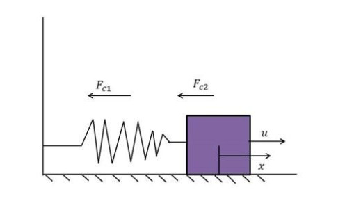
The finite-time $ {H_\infty } $ performance of the interval type-2 Takagi-Sugeno fuzzy system (IT2 T-S) in presence of immeasurable states and input saturation is investigated. At first, an observer associated with IT2 T-S states is considered to address the problem of immeasurable states. After that, the input saturation is described based on the polyhedron model, and accordingly, a robust $ {H_\infty } $ observer-based finite-time controller is proposed via non-PDC algorithm. Then, on the basis of the Lyapunov function method and LMIs theory, the sufficient conditions for the finite time stability of fuzzy systems are derived. At last, the feasibility of the designed algorithm is verified by two examples of the nonlinear mass-spring-damping system and tunnel diode circuit system, respectively.
Citation: Chuang Liu, Jinxia Wu, Weidong Yang. Robust $ {H}_{\infty} $ output feedback finite-time control for interval type-2 fuzzy systems with actuator saturation[J]. AIMS Mathematics, 2022, 7(3): 4614-4635. doi: 10.3934/math.2022257

Related Papers:

Abstract

The finite-time $ {H_\infty } $ performance of the interval type-2 Takagi-Sugeno fuzzy system (IT2 T-S) in presence of immeasurable states and input saturation is investigated. At first, an observer associated with IT2 T-S states is considered to address the problem of immeasurable states. After that, the input saturation is described based on the polyhedron model, and accordingly, a robust $ {H_\infty } $ observer-based finite-time controller is proposed via non-PDC algorithm. Then, on the basis of the Lyapunov function method and LMIs theory, the sufficient conditions for the finite time stability of fuzzy systems are derived. At last, the feasibility of the designed algorithm is verified by two examples of the nonlinear mass-spring-damping system and tunnel diode circuit system, respectively.

References

[1]	X. D. Li, J. H. Shen, H. Akca, R. Rakkiyappan, LMI-based stability for singularly perturbed nonlinear impulsive differential systems with delays of small parameter, Appl. Math. Comput., 250 (2015), 798–804. https://doi.org/10.1016/j.amc.2014.10.113 doi: 10.1016/j.amc.2014.10.113
[2]	X. D. Li, P. Li, Stability of time-delay systems with impulsive control involving stabilizing delays, Automatica, 124 (2021), 109336. https://doi.org/10.1016/j.automatica.2020.109336 doi: 10.1016/j.automatica.2020.109336
[3]	D. Yang, X. D. Li, J. L. Qiu, Output tracking control of delayed switched systems via state-dependent switching and dynamic output feedback, Nonlinear Anal-Hybri., 32 (2019), 294–305. https://doi.org/10.1016/j.nahs.2019.01.006 doi: 10.1016/j.nahs.2019.01.006
[4]	Y. Chen, J. X. Wu, J. Lan, Study on reasonable initialization enhanced Karnik-Mendel algorithms for centroid type-reduction of interval type-2 fuzzy logic systems, AIMS Mathematics, 5 (2020), 6149–6168. https://doi.org/10.3934/math.2020395 doi: 10.3934/math.2020395
[5]	Y. Chen, J. X. Wu, J. Lan, Study on weighted-based noniterative algorithms for centroid type-reduction of interval type-2 fuzzy logic systems, AIMS Mathematics, 5 (2020), 7719–7745. https://doi.org/10.3934/math.2020494 doi: 10.3934/math.2020494
[6]	H. K. Lam, L. D. Seneviratne, Stability analysis of interval type-2 fuzzy-model-based control systems, IEEE T. Syst. Man Cy. B, 38 (2008), 617–628. https://doi.org/10.1109/TSMCB.2008.915530 doi: 10.1109/TSMCB.2008.915530
[7]	T. Zhao, S. Y. Dian, State feedback control for interval type-2 fuzzy systems with time-varying delay and unreliable communication links, IEEE T. Fuzzy Syst., 26 (2018), 951–966. https://doi.org/10.1109/TFUZZ.2017.2699947 doi: 10.1109/TFUZZ.2017.2699947
[8]	L. Sheng, X. Y. Ma, Stability analysis and controller design of interval type-2 fuzzy systems with time delay, Int. J. Syst. Sci., 45 (2014), 977–993. https://doi.org/10.1080/00207721.2012.743056 doi: 10.1080/00207721.2012.743056
[9]	R. Kavikumar, R. Sakthivel, O. M. Kwon, B. Kaviarasan, Faulty actuator-based control synthesis for interval type-2 fuzzy systems via memory state feedback approach, Int. J. Syst. Sci., 51 (2020), 2958–2981. https://doi.org/10.1080/00207721.2020.1804643 doi: 10.1080/00207721.2020.1804643
[10]	H. K. Lam, H. Y. Li, C. Deters, E. L. Secco, H-A. Wurdemann, K. Althoefer, Control design for interval type-2 fuzzy systems under imperfect premise matching, IEEE T. Ind. Electron., 61 (2014), 956–968. https://doi.org/10.1109/TIE.2013.2253064 doi: 10.1109/TIE.2013.2253064
[11]	H. Y. Li, X. J. Sun, L. G. Wu, H. K. Lam, State and output feedback control of interval type-2 fuzzy systems with mismatched membership functions, IEEE T. Fuzzy Syst., 23 (2015), 1943–1957. https://doi.org/10.1109/TFUZZ.2014.2387876 doi: 10.1109/TFUZZ.2014.2387876
[12]	W. Zheng, Z. M. Zhang, H. B. Wang, H. R. Wang, Robust $H_\infty$ dynamic output feedback control for interval type-2 T-S fuzzy multiple time-varying delays systems with external disturbance, J. Franklin I., 357 (2020), 3193–3218. https://doi.org/10.1016/j.jfranklin.2019.03.039 doi: 10.1016/j.jfranklin.2019.03.039
[13]	W. T. Song, S. C. Tong, Observer-based fuzzy event-triggered control for interval type-2 fuzzy systems, Int. J. Fuzzy Syst., (2021). https://doi.org/10.1007/s40815-021-01114-w
[14]	O. Uncu, I. B. Turksen, Discrete interval type 2 fuzzy system models using uncertainty in learning parameters, IEEE T. Fuzzy Syst., 15 (2007), 90–106. https://doi.org/10.1109/TFUZZ.2006.889765 doi: 10.1109/TFUZZ.2006.889765
[15]	Y. B. Gao, H. Y. Li, L. G. Wu, H. R. Karimi, H. K. Lam, Optimal control of discrete-time interval type-2 fuzzy-model-based systems with D-stability constraint and control saturation, Signal Process., 120 (2016), 409–421. https://doi.org/10.1016/j.sigpro.2015.09.007 doi: 10.1016/j.sigpro.2015.09.007
[16]	Q. Zhou, D. Liu, Y. B. Cao, H. K. Lam, R. Sakthivel, Interval type-2 fuzzy control for nonlinear discrete-time systems with time-varying delays, Neurocomputing, 157 (2015), 22–32. https://doi.org/10.1016/j.neucom.2015.01.042 doi: 10.1016/j.neucom.2015.01.042
[17]	T. Zhao, S. Y. Dian, Delay-dependent stabilization of discrete-time interval type-2 T- S fuzzy systems with time-varying delay, J. Franklin I., 354 (2017), 1542–1567. https://doi.org/10.1016/j.jfranklin.2016.12.002 doi: 10.1016/j.jfranklin.2016.12.002
[18]	Y. Zeng, H. K. Lam, B. Xiao, L. G. Wu, $L_2 - {L_\infty }$ control of discrete-time state-delay interval type-2 fuzzy systems via dynamic output feedback, IEEE T. Cybernetics, (2020), 1–11. http://dx.doi.org/10.1109/TCYB.2020.3024754
[19]	W. T. Song, S. C. Tong, Fuzzy decentralized output feedback event-triggered control for interval type-2 fuzzy systems with saturated inputs, Inform. Sciences, 575 (2021), 639–653. https://doi.org/10.1016/j.ins.2021.07.070 doi: 10.1016/j.ins.2021.07.070
[20]	F. Amato, M. Ariola, P. Dorato, Finite-time control of linear systems subject to parametric uncertainties and disturbances, Automatica, 37 (2001), 1459–1463. https://doi.org/10.1016/S0005-1098(01)00087-5 doi: 10.1016/S0005-1098(01)00087-5
[21]	Y. Li, L. Liu, G. Feng, Finite-time stabilization of a class of T-S fuzzy systems, IEEE T. Fuzzy Syst., 25 (2017), 1824–1829. https://doi.org/10.1109/TFUZZ.2016.2612301 doi: 10.1109/TFUZZ.2016.2612301
[22]	L. Han, C. Y. Qiu, J. Xiao, Finite-time ${H_\infty }$ control Synthesis for nonlinear switched systems using T-S fuzzy model, Neurocomputing, 171 (2016), 156–170. https://doi.org/10.1016/j.neucom.2015.06.028 doi: 10.1016/j.neucom.2015.06.028
[23]	M. Chen, J. Sun, ${H_\infty }$ finite time control for discrete time-varying system with interval time-varying delay, J. Franklin I., 355 (2018), 5037–5057. https://doi.org/10.1016/j.jfranklin.2018.05.031 doi: 10.1016/j.jfranklin.2018.05.031
[24]	Y. Q. Zhang, Y. Shi, P. Shi, Robust and non-fragile finite-time ${H_\infty }$ control for uncertain Markovian jump nonlinear systems, Appl. Math. Comput., 279 (2016), 125–138. https://doi.org/10.1016/j.amc.2016.01.012 doi: 10.1016/j.amc.2016.01.012
[25]	Y. Q. Zhang, Y. Shi, P. Shi, Resilient and robust finite-time ${H_\infty }$ control for uncertain discrete-time jump nonlinear systems, Appl. Math. Model., 49 (2017), 612–629. https://doi.org/10.1016/j.apm.2017.02.046 doi: 10.1016/j.apm.2017.02.046
[26]	Y. Q. Zhang, C. X. Liu, X. W. Mu, Robust finite-time ${H_\infty }$ control of singular stochastic systems via static output feedback, Appl. Math. Comput., 218 (2012), 5629–5640. https://doi.org/10.1016/j.amc.2011.11.057 doi: 10.1016/j.amc.2011.11.057
[27]	Y. Q. Zhang, P. Shi, S. K. Nguang, Observer-based finite-time ${H_\infty }$ control for discrete singular stochastic systems, Appl. Math. Lett., 38 (2014), 115–121. https://doi.org/10.1016/j.aml.2014.07.010 doi: 10.1016/j.aml.2014.07.010
[28]	T. Zhao, J. H. Liu, S. Y. Dian, Finite-time control for interval type-2 fuzzy time-delay systems with norm-bounded uncertainties and limited communication capacity, Inform. Sciences, 483 (2019), 153–173. https://doi.org/10.1016/j.ins.2019.01.044 doi: 10.1016/j.ins.2019.01.044
[29]	R. Kavikumar, R. Sakthivel, O. M. Kwon, B. Kaviarasan, Finite-time boundedness of interval type-2 fuzzy systems with time delay and actuator faults, J. Franklin I., 356 (2019), 8296–8324. https://doi.org/10.1016/j.jfranklin.2019.07.031 doi: 10.1016/j.jfranklin.2019.07.031
[30]	N. N. Rong, Z. S. Wang, H. G. Zhang, Finite-time stabilization for discontinuous interconnected delayed systems via interval type-2 T-S fuzzy model approach, IEEE T. Fuzzy Syst., 27 (2019), 249–261. https://doi.org/10.1109/TFUZZ.2018.2856181 doi: 10.1109/TFUZZ.2018.2856181
[31]	Z. S. Wang, N. N. Rong, H. G. Zhang, Finite-time decentralized control of IT2 T-S fuzzy interconnected systems with discontinuous interconnections, IEEE T. Cybernetics, 49 (2019), 3547–3556. https://doi.org/10.1109/TCYB.2018.2848626 doi: 10.1109/TCYB.2018.2848626
[32]	Y. Y. Cao, Z. L. Lin, Robust stability analysis and fuzzy-scheduling control for nonlinear systems subject to actuator saturation, IEEE T. Fuzzy Syst., 11 (2003), 57–67. https://doi.org/10.1109/TFUZZ.2002.806317 doi: 10.1109/TFUZZ.2002.806317
[33]	D. Saifia, C. Mohammed, S. Labiod, T. M. Guerra, Robust ${H_\infty }$ static output feedback stabilization of T-S fuzzy systems subject to actuator saturation, Int. J. Control Autom., 10 (2012), 613–622. https://doi.org/10.1007/s12555-012-0319-3 doi: 10.1007/s12555-012-0319-3
[34]	F. W. Yang, Z. D. Wang, Y. S. Hung, M. Gani, Robust ${H_\infty }$ control for networked systems with random communication delays, IEEE T. Automat. Contr., 51 (2006), 511–518. https://doi.org/10.1109/TAC.2005.864207 doi: 10.1109/TAC.2005.864207

Reader Comments

Your name:*

Email:*
© 2022 the Author(s), licensee AIMS Press. This is an open access article distributed under the terms of the Creative Commons Attribution License (http://creativecommons.org/licenses/by/4.0)