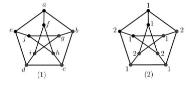
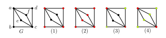
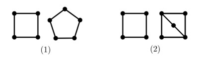
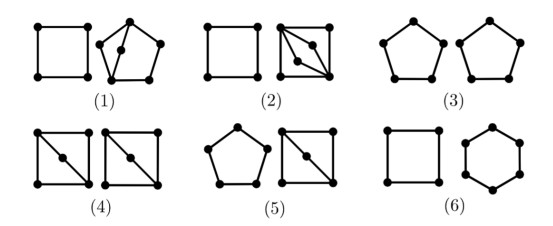
Let G be a vertex-colored graph. A vertex cut S of G is called a monochromatic vertex cut if the vertices of S are colored with the same color. A graph G is monochromatically vertex-disconnected if any two nonadjacent vertices of G have a monochromatic vertex cut separating them. The monochromatic vertex disconnection number of G, denoted by mvd(G), is the maximum number of colors that are used to make G monochromatically vertex-disconnected. In this paper, the connection between the graph parameters are studied: mvd(G), connectivity and block decomposition. We determine the value of mvd(G) for some well-known graphs, and then characterize G when n−5≤mvd(G)≤n and all blocks of G are minimally 2-connected triangle-free graphs. We obtain the maximum size of a graph G with mvd(G)=k for any k. Finally, we study the Erdős-Gallai-type results for mvd(G), and completely solve them.
Citation: Miao Fu, Yuqin Zhang. Results on monochromatic vertex disconnection of graphs[J]. AIMS Mathematics, 2023, 8(6): 13219-13240. doi: 10.3934/math.2023668
[1] | Yanping Yang, Yang Wang, Juan Liu . List vertex arboricity of planar graphs without 5-cycles intersecting with 6-cycles. AIMS Mathematics, 2021, 6(9): 9757-9769. doi: 10.3934/math.2021567 |
[2] | Yindi Weng . Bounds and complexity results of rainbow vertex-disconnection colorings. AIMS Mathematics, 2025, 10(3): 5960-5970. doi: 10.3934/math.2025272 |
[3] | Jianwei Du, Xiaoling Sun . On the graph connectivity and the variable sum exdeg index. AIMS Mathematics, 2021, 6(1): 607-622. doi: 10.3934/math.2021037 |
[4] | Weisheng Zhao, Ying Li, Ruizhi Lin . The existence of a graph whose vertex set can be partitioned into a fixed number of strong domination-critical vertex-sets. AIMS Mathematics, 2024, 9(1): 1926-1938. doi: 10.3934/math.2024095 |
[5] | Gohar Ali, Martin Bača, Marcela Lascsáková, Andrea Semaničová-Feňovčíková, Ahmad ALoqaily, Nabil Mlaiki . Modular total vertex irregularity strength of graphs. AIMS Mathematics, 2023, 8(4): 7662-7671. doi: 10.3934/math.2023384 |
[6] | Gaixiang Cai, Fengru Xiao, Guidong Yu . The identification numbers of lollipop graphs. AIMS Mathematics, 2025, 10(4): 7813-7827. doi: 10.3934/math.2025358 |
[7] | Li-Ming Yeh . Lipschitz estimate for elliptic equations with oscillatory coefficients. AIMS Mathematics, 2024, 9(10): 29135-29166. doi: 10.3934/math.20241413 |
[8] | Baolin Ma, Chao Yang . Distinguishing colorings of graphs and their subgraphs. AIMS Mathematics, 2023, 8(11): 26561-26573. doi: 10.3934/math.20231357 |
[9] | Ningge Huang, Lily Chen . AVD edge-colorings of cubic Halin graphs. AIMS Mathematics, 2023, 8(11): 27820-27839. doi: 10.3934/math.20231423 |
[10] | Xue Yu, Qingshan Zhang . Orientable vertex transitive embeddings of Kp. AIMS Mathematics, 2023, 8(7): 15024-15034. doi: 10.3934/math.2023767 |
Let G be a vertex-colored graph. A vertex cut S of G is called a monochromatic vertex cut if the vertices of S are colored with the same color. A graph G is monochromatically vertex-disconnected if any two nonadjacent vertices of G have a monochromatic vertex cut separating them. The monochromatic vertex disconnection number of G, denoted by mvd(G), is the maximum number of colors that are used to make G monochromatically vertex-disconnected. In this paper, the connection between the graph parameters are studied: mvd(G), connectivity and block decomposition. We determine the value of mvd(G) for some well-known graphs, and then characterize G when n−5≤mvd(G)≤n and all blocks of G are minimally 2-connected triangle-free graphs. We obtain the maximum size of a graph G with mvd(G)=k for any k. Finally, we study the Erdős-Gallai-type results for mvd(G), and completely solve them.
Connectivity is perhaps the most fundamental graph theoretic subject, in both the combinatorial and network science senses. To expand its application area, connectivity is strengthened through tasks such as requiring graph coloring, Hamiltonicity [13] and conditional connectivity [11].
In 2008, Chartrand et al. [5,6] introduced an interesting way, i.e., the rainbow k-connection, to strengthen conventional connectivity. An edge-colored graph G is called rainbow k-connected if any pair of vertices are connected by k internally vertex-disjoint rainbow paths, where a rainbow path is a path with edges that all carry different colors. This concept comes from the communication of information between agencies of the government, and it is also applied to communication networks. More developments for variants of rainbow k-connectivity of different graph families can be found, e.g., in the survey [18].
Moving away from deterministic graphs, similar results have also been investigated for random graph models (see [7,22]). In particular, a multiplex approach to cope with rainbow-related concepts has recently attracted increasing research attention in random settings. For example, Shang [23] approached rainbow k-connectivity by considering an alternative random network with multiple layers. Meanwhile, many colored versions of connectivity parameters have been introduced in recent years. For example, the monochromatic connection introduced by Caro and Yuster [3] in 2011 is defined from the monochromatic version; the monochromatic vertex connection introduced by Cai, Li and Wu [4] in 2018 is defined from the vertex version. For more results, we refer the reader to [10,14,19,23].
There are two ways to study the connectivity, one using paths and the other using vertex cuts. These concepts mentioned above use paths, so it is natural to consider monochromatic vertex cuts. Let G be a vertex-colored graph. A vertex cut S is called a monochromatic vertex cut if the vertices of S are colored with the same color, and a monochromatic x-y vertex cut is a monochromatic vertex cut that separates x and y. Obviously, if x is adjacent to y, there is no x-y vertex cut, so we only need to consider nonadjacent vertices in the sequel. Then, G is called monochromatically vertex-disconnected if any two nonadjacent vertices of G have a monochromatic vertex cut separating them; the corresponding coloring is called monochromatic vertex-disconnection coloring (MVD-coloring for short). The monochromatic vertex disconnection number of G, denoted by mvd(G), is the maximum number of colors that are used to make G monochromatically vertex-disconnected. An MVD-coloring with mvd(G) colors is called an mvd-coloring of G.
In addition to being a natural combinatorial measure, our parameter can also be applied to communication networks. Suppose that G represents a network (e.g., a cellular network) where messages can be transmitted between any two vertices. To intercept messages (e.g., to prevent the transmission of error messages), each vertex is equipped with an interceptor that requires a fixed password (color) to be turned on. There is a fixed interception passphrase between any two different vertices. Entering this passphrase at the vertex cut where the password matches will turn on these interceptors and intercept the message between the two vertices. To enhance system security, the number of passwords should be as large as possible. This number is precisely mvd(G).
In this paper, the connection between graph parameters are studied: mvd(G) and connectivity κ(G). We obtain the following results in Section 2:
Theorem 1.1. If G is a connected non-complete graph, then 1≤mvd(G)≤n−κ+(G)+1≤n−κ(G)+1. The upper bound is tight.
Further, for the minimally 2-connected graph of order n≥4, we give a new upper bound:
Theorem 1.2. If G is a minimally 2-connected graph of order n≥4, then mvd(G)≤⌊n2⌋. The bound is tight.
For the graph G with κ(G)=1, mvd-coloring, a global property of G, is transformed into a local property of each block, which greatly simplifies the original problem:
Theorem 1.3. If κ(G)=1 and G has r blocks B1, …,Br, then mvd(G)=(r∑i=1mvd(Bi))−r+1.
In Section 3, we focus on the value of mvd(G) for some well-known graphs with κ(G)≥2 and obtain several classes of graphs with mvd(G)=k, where k∈{1,2,n}. Moreover, we completely characterize G when n−5≤mvd(G)≤n and all blocks of G are minimally 2-connected triangle-free graphs.
The Erdős-Gallai theorem [8] originated in 1959 and is an interesting problem in extremal graph theory, where the Erdős-Gallai-type result aims at determining the maximum or minimum value of a graph parameter with some given properties. For a graph parameter, it is always interesting and challenging to get the Erdős-Gallai-type results; see [1,9,15,16,20] for more such results on various kinds of graph parameters. In Section 4, we study two kinds of Erdős-Gallai-type problems for our parameter mvd(G).
Problem Ⅰ. Given two positive integers n and k with 1≤k≤n, compute the minimum integer fv(n,k) such that, for any graph G of order n, if |E(G)|≥fv(n,k), then mvd(G)≥k.
Problem Ⅱ. Given two positive integers n and k with 1≤k≤n, compute the maximum integer gv(n,k) such that, for any graph G of order n, if |E(G)|≤gv(n,k), then mvd(G)≤k.
By Theorem 1.3, for any tree G of order n, we have mvd(G)=n, so gv(n,k) does not exist for 1≤k≤n−1. Since mvd(Kn)=n, where Kn is a complete graph, gv(n,n)=n(n−1)2. The result of Problem Ⅰ is shown below.
Theorem 1.4. Given two positive integers n and k with n≥5 and 1≤k≤n,
fv(n,k)={n−1,k=1,n(n−1)2−1,2≤k≤3,n(n−1)2,4≤k≤n. |
Moreover, we obtain the maximum size of G with mvd(G)=k for any k.
Theorem 1.5. Given two positive integers n and k with n>4 and 1≤k≤n, the maximum size of a connected graph G of order n with mvd(G)=k is
|E(G)|max={n(n−1)2−2,k=1 and n≥5,7,k=2 and n=5,n(n−1)2−4,k=2 and n≥6,n(n−1)2−k+2,3≤k≤n−1,n(n−1)2,k=n. |
All graphs considered in this paper are simple, connected, finite and undirected. We follow the terminology and notation of Bondy and Murty [2]. Let n=|G| be the order of G, and let |E(G)| be the size of G. For D⊆E(G), G−D is the graph obtained by removing D from G. For S⊆V(G), G−S is the graph obtained by removing S and the edges incident to the vertices of S from G. We use [r] to denote the set {1,2,…,r}. For a vertex-coloring τ of G, τ(v) is the color of vertex v, τ(G) is the set of colors used in G and |τ(G)| is the number of colors in τ(G). If H is a subgraph of G, then the part of the coloring of τ on H is called τ-restricted on H. To show the connection between mvd(G) and connectivity κ(G), we need the following lemma:
Lemma 2.1. If τ is an MVD-coloring of G, then τ restricted on G[S] is also an MVD-coloring of G[S].
Proof. Let the coloring of τ restricted on G[S] be denoted as τ′, and let x and y be two nonadjacent vertices of G[S]. If D is a monochromatic x-y vertex cut of G, then D′=D∩V(G[S]) is a monochromatic x-y vertex cut in G[S]. Otherwise, if there is an x,y-path P in G[S]−D′, then P is also in G−D, which is a contradiction. Thus, τ′ is an MVD-coloring of G[S].
Proof of Theorem 1.1. G is a non-complete graph and x and y are two nonadjacent vertices of G. Let κ(x,y) be the minimum size of an x-y vertex cut, and let κ+(G) be the upper bound of the function κ(x,y). Obviously, mvd(G)≥1. For the upper bound, assume that S is a monochromatic x-y vertex cut. Therefore, mvd(G)≤1+(n−|S|)≤n−κ(x,y)+1. Thus, mvd(G)≤n−κ+(G)+1≤n−κ(G)+1.
Tight example 1: Let G be a graph obtained by adding k edges to Kn−1 from a vertex v outside Kn−1, where k∈[n−2]. Clearly, κ(G)=k. Define a vertex-coloring τ of G: V(G)→[n−k+1] such that τ(G−N(v))→[n−k] and τ(N(v))=n−k+1. If x and y are two nonadjacent vertices in G, then either x or y is v, i.e., v=x. Since τ(N(v))=n−k+1, N(v) is a monochromatic v-y vertex cut and τ is a MVD-coloring of G. So, mvd(G)≥n−k+1. It follows that mvd(G)=n−κ(G)+1. The upper bound is tight.
A graph G is minimally 2-connected (minimal block) if G is 2-connected but G−{e} is not 2-connected for every e∈E(G). Before proving Theorem 1.2, we need more preparation: a nest sequence of graphs is a sequence G0,G1,…,Gt of graphs such that Gi⊂Gi+1,0≤i<t; an ear decomposition of a 2-connected graph G is a nest sequence G0,G1,…,Gt of 2-connected subgraphs of G satisfying the following conditions: (ⅰ) G0 is a cycle of G; (ⅱ) Gi+1=Gi∪Pi, where Pi is an ear of Gi, 0≤i<t; (ⅲ) Gt=G.
Lemma 2.2. [17] Let G be a minimally 2-connected graph, and G is not a cycle. Then, G has an ear decomposition G0,G1,…,Gt (t≥1) satisfying the following conditions:
(i) Gi+1=Gi∪Pi (0≤i<t), where Pi is an ear of Gi in G and at least one vertex of Pi has degree two in G;
(ii) each of the two internally disjoint paths in G0 between the endpoints of P0 has at least one vertex with degree two in G.
Lemma 2.3. [21] If G is a minimally 2-connected graph of order n≥4, then G contains no triangles.
Lemma 2.4. If G is a cycle of order n≥4, then mvd(G)=⌊n2⌋.
Proof. Let G=v1e1…vnenv1. Define a vertex-coloring τ:V(G)→[⌊n2⌋] such that, if j≡i (mod ⌊n2⌋), then τ(vj)=i, where i∈[⌊n2⌋] and j∈[n]. It can be shown that, for any two nonadjacent vertices x and y, there is a monochromatic x-y vertex cut. So, τ is an MVD-coloring and mvd(G)≥⌊n2⌋.
If, on the contrary, for n≥4, mvd(G)≥⌊n2⌋+1 and τ is an mvd-coloring of G with |τ(G)|=mvd(G)≥⌊n2⌋+1, then there must be a color that colors only one vertex vi; otherwise, we have V(G)≥2|τ(G)|≥2(⌊n2⌋+1)≥n+1. Since κ(G)=2, the monochromatic vi−1-vi+1 vertex cut must contain vi and some vertex vj in G−{vi−1,vi,vi+1}. However, τ(vi)≠τ(vj), which contradicts the fact that τ is an mvd-coloring. Thus, mvd(G)=⌊n2⌋.
Proof of Theorem 1.2. We make the following claim:
Claim 1: If G is a 2-connected triangle-free graph and every ear Pi (0≤i<t) has internal vertices, then mvd(G)≤⌊n2⌋.
Let F={G0,G1,…,Gt} be an ear decomposition of G. We use induction on |F|. By Lemma 2.4, the claim holds for |F|=1. If |F|=t+1>1, let τ be an mvd-coloring of G. Since |Pt−1|≥3, Gt−1 is a connected vertex-induced subgraph of G. By Lemma 2.1, τ restricted on Gt−1 is an MVD-coloring of Gt−1. By induction, we have
|τ(Gt−1)|≤mvd(Gt−1)≤⌊|Gt−1|2⌋=⌊n−|Pt−1|+22⌋. |
Suppose that the endpoints of Pt−1 are a and b and L is the shortest a,b-path in Gt−1. Since Pt−1 is the last ear, cycle C=L∪Pt−1 is a connected vertex-induced subgraph of G and τ restricted on C is an MVD-coloring of C. Then, there are at most |Pt−1|−2 vertices that are assigned colors in τ(G)−τ(Gt−1). Since |C|≥4, each color in τ(G)−τ(Gt−1) colors at least two internal vertices of Pt−1. Otherwise, if j∈τ(G)−τ(Gt−1) and only colors one internal vertex of Pt−1, say xj, then xj−1 and xj+1 are two nonadjacent vertices of G and the monochromatic xj−1-xj+1 vertex cut must contain xj and another vertex, which is a contradiction. Then, |τ(G)−τ(Gt−1)|≤⌊|Pt−1|−22⌋. So,
mvd(G)=|τ(G)|=|τ(Gt−1)|+|τ(G)−τ(Gt−1)|≤⌊n−|Pt−1|+22⌋+⌊|Pt−1|−22⌋≤⌊n2⌋. |
Above all, mvd(G)≤⌊n2⌋.
By Lemmas 2.2 and 2.3, if G is not a cycle, then there is an ear decomposition satisfying the conditions in Claim 1. Thus, mvd(G)≤⌊n2⌋.
Tight example 2: If G is a cycle, then, according to Lemma 2.4, we have mvd(G)=⌊n2⌋. The bound is tight.
A block is a maximal connected subgraph of G that has no cut-vertex. Every block of a nontrivial connected graph is either K2 or a 2-connected subgraph, called trivial and nontrivial, respectively. To show the connection between mvd(G) and block decomposition, we need the following result:
Theorem 2.1. Let G be a connected graph with r blocks. Then, τ is an mvd-coloring of G if and only if τ restricted on each block is an mvd-coloring of each block and the colors of different blocks are different except at the cut vertices.
Proof. Let {B1,…,Br} be the block decomposition of G. Let τ be a vertex-coloring of G, and let τi be the coloring of τ restricted on Bi, i∈[r]. If G has no cut vertex, then G=B1 and the result follows. Now, we assume that G has at least one cut vertex:
Claim 1: τ is an MVD-coloring of G if and only if τ restricted on each block is an MVD-coloring of each block.
Since each block is a vertex-induced subgraph of G, the necessity is obvious by Lemma 2.1. Now, let τi be an MVD-coloring of Bi, where i∈[r]. For any two nonadjacent vertices x and y in G, if there is a block, say B1, which contains both x and y, then any monochromatic x-y vertex cut in B1 is also a monochromatic x-y vertex cut in G. If x and y are in different blocks, then there is exactly one internally disjoint x,y-path containing at least one cut vertex v. The vertex v is a monochromatic x-y vertex cut in G. Thus, τ is an MVD-coloring of G.
Next, let τi be an mvd-coloring of Bi satisfying that, if Bi∩Bj=v, then τi(Bi)∩τj(Bj)=τi(v)=τj(v), and if Bi∩Bj=∅, then τi(Bi)∩τj(Bj)=∅, where i,j∈[r] and i≠j. Then, τ is an MVD-coloring of G by Claim 1. We claim that τ is an mvd-coloring of G. Otherwise, there is an mvd-coloring τ′ of G satisfying |τ′(G)|>|τ(G)|. Let the coloring of τ′ restricted on Bi be τ′i, which is an MVD-coloring of Bi by Claim 1. Then, for any i∈[r], |τ′i(Bi)|≤|τi(Bi)|, which contradicts |τ′(G)|>|τ(G)|. Thus, τ is an mvd-coloring of G.
Now, we prove the necessity of the theorem. Let τ be an mvd-coloring of G. According to Claim 1, τi is an MVD-coloring of Bi, i∈[r]. Similar to the proof of Claim 1, it can be shown that, if Bi∩Bj=v, then τi(Bi)∩τj(Bj)=τi(v)=τj(v), and if Bi∩Bj=∅, then τi(Bi)∩τj(Bj)=∅, where i,j∈[r] and i≠j. We only need to prove that τi is an mvd-coloring of Bi, i∈[r]. If τ1 is not an mvd-coloring of B1, then there must be an mvd-coloring τ′1 of B1 satisfying that all colors in τ′1(B1) are unused colors, except for those owned by cut vertices. It follows that |τ′1(B1)|>|τ1(B1)| and |τ′(G)|>|τ(G)|. According to the sufficiency of Claim 1, τ′ is an MVD-coloring of G, which contradicts the maximality of τ.
Proof of Theorem 1.3. Let G be a connected graph with blocks B1,B2,…,Br, and let τ be an mvd-coloring of G. We use induction on r. The result holds for r=1. If r>1, then G is not 2-connected; we know that there is a block, say Br, containing only one cut vertex, say v. Let G′=G−(V(Br)−{v}). Then, G′ is a connected graph with blocks B1,B2,…,Br−1. By Theorem 2.1, τ restricted on G′ is an mvd-coloring of G′, and, combined with the induction hypothesis, we have |τ(G′)|=mvd(G′)=(∑r−1i=1mvd(Bi))−(r−1)+1. According to Theorem 2.1, τ restricted on Br is an mvd-coloring of Br and τ(Br)∩τ(G′)=τ(v). So, we deleted |mvd(Br)|−1 colors from τ(G) to obtain τ(G′); mvd(G) is as desired.
If G and H are vertex-disjoint, then let G∨H denote the join of G and H, which is obtained from G and H by adding edges {xy:x∈V(G),y∈V(H)}. If Cn−1 is a cycle of order n−1, then Wn=Cn−1∨K1 is called a wheel graph. We first show several classes of graphs with mvd(G)=k, where k∈{1,2,n}.
Theorem 3.1. If G is one of the following graphs, then mvd(G)=1.
(i) G is a wheel graph other than W4;
(ii) G=Kn1,…,nk is a complete k-partite graph with nk, nk−1≥2 and k>2.
(1) Let G=Wn=Cn−1∨K1, where cycle Cn−1=v1v2…vn−1v1 and K1=v. It is known that mvd(W4)=mvd(K4)=4. We claim that mvd(Wn)=1 for n>4.
Let τ be an mvd-coloring of Wn, say τ(v)=1. Since n>4, v1 and v3 are two nonadjacent vertices with three internally disjoint v1,v3-paths, namely, v1v2v3, v1vv3 and v1vn−1vn−2⋯v4v3. Since κ(Wn)=3, any monochromatic v1-v3 vertex cut must contain the vertex set {v2,v,vi}, where vi∈{vn−1,vn−2,…,v4}, so τ(v2)=1. Similarly, v2 and v4 are two nonadjacent vertices, and we get τ(v3)=1. Repeat operations above until all vertices of Cn−1 are colored, and we get τ(v)=τ(v1)=τ(v2)=⋯=τ(vn−1)=1. Therefore, mvd(Wn)=1 for n>4.
(2) Let G=Kn1,n2,…,nk be a complete k-partite graph of order n, where k≥2 and 1≤n1≤n2≤⋯≤nk. Let V1,V2,…,Vk be the vertex-partition sets of G with |Vi|=ni, where i∈[k]. There are four cases below.
Case 1. ni=1 for i∈[k]; then, mvd(G)=mvd(Kn)=n.
Case 2. ni=1 for i∈[k−1], and nk≥2:
Define a vertex-coloring τ:V(G)→[n−k+2] such that τ(Vk)→[n−k+1] and τ(Vi)=n−k+2 for i∈[k−1]. If x and y are two nonadjacent vertices in G, then x, y∈Vk and V(G)−Vk is a monochromatic x-y vertex cut in G. Thus, τ is an MVD-coloring of G and mvd(G)≥n−k+2. On the other hand, since any two vertices in Vk have k−1 internally disjoint paths, according to Theorem 1.1, mvd(G)≤n−κ+(G)+1=n−k+2.
Case 3. k>2 and nk≥nk−1≥2:
x and y are nonadjacent. If x, y∈Vk−1, then any x-y vertex cut must contain V(G)−Vk−1. So, V(G)−Vk−1 are assigned the same color. Similarly, if x, y∈Vk, then V(G)−Vk are assigned the same color. Since k>2, the sets V(G)−Vk−1 and V(G)−Vk−1 intersect. Then, mvd(G)=1.
Case 4. k=2, n2≥n1≥2:
Similarly, since k=2, the sets V(G)−V1 and V(G)−V2 are disjoint; then, mvd(Kn1,n2)=2.
The Cartesian product of G and H, written as G◻H, is the graph with the vertex set V(G)×V(H), specified by putting (u,v) adjacent to (u′,v′) if and only if either u=u′ and vv′∈E(H), or v=v′ and uu′∈E(G). If Pn is a path with order n, then Pm◻Pn is called the m-by-n grid.
Theorem 3.2. If G is one of the following graphs, then mvd(G)=2.
(i) G=Pm◻Pn is a nontrivial grid other than P1◻Pn with n>2;
(ii) G is a Petersen graph.
Proof. (1) Let G=Pm◻Pn and define xi,j to be the vertex in the i-th row and j-th column, where i∈[m] and j∈[n]. It is known that mvd(P1◻Pn)=mvd(Pn)=n. Then, mvd(P1◻P2)=2 and mvd(P1◻Pn)>2 for n>2. We claim that mvd(Pm◻Pn)=2 for m,n≥2.
Define a vertex-coloring τ of G: V(G)→[2] such that τ(xi,j)=1 if i+j is even and τ(xi,j)=2 if i+j is odd. For any vertex x in G, the set N(x) is monochromatic. Thus, for any two nonadjacent vertices x and y in G, N(x) is a monochromatic x-y vertex cut. So, mvd(G)≥2.
Now, we prove that mvd(G)=2. Any MVD-coloring of a 4-cycle can have only two cases, where one is trivial and the other is to assign colors 1 and 2 to the four vertices of the 4-cycle alternately. Suppose that mvd(G)>2 and τ is an mvd-coloring of G. By Lemma 2.1, τ restricted on each 4-cycle G[xi,j,xi,j+1, xi+1,j+1,xi+1,j] is an MVD-coloring, given 1≤i<m,1≤j<n, which contradicts that mvd(G)>2. Therefore, mvd(Pm◻Pn)=2 for m,n≥2.
(2) Define a vertex-coloring τ of G: V(G)→[2] as shown in Figure 1(2). For any two nonadjacent vertices x and y, there is only one common neighbor, say z. Suppose that τ(z)=t; it can be shown that the set of all vertices colored by t, except x and y, is a monochromatic x-y vertex cut. Thus, τ is an MVD-coloring of G and mvd(G)≥2. We prove that mvd(G)=2 below.
Any MVD-coloring of C5 can only be two cases, where one is trivial and the other is to assign colors 1 and 2 to the five vertices of C5 alternately. At least two adjacent vertices in C5 have the same color. Suppose that mvd(G)>2 and τ is an mvd-coloring of G. Let the four 5-cycles of G be G1=G[a,b,c,d,e],G2=G[c,d,i,f,h],G3=G[a,b,c,h,f] and G4=G[f,h,j,g,i]. Since τ restricted on G1 is an MVD-coloring, there are two cases.
Case 1. G1 is colored nontrivially.
Suppose that τ(a)=τ(c)=τ(d)=1 and τ(b)=τ(e)=2. Then, τ restricted on G2 is an MVD-coloring. If G2 is colored trivially, i.e., τ(f)=τ(h)=τ(i)=1, it is obvious that τ is not an MVD-coloring restricted on G3. By Lemma 2.1, τ is not an MVD-coloring of G, which contradicts that τ is an mvd-coloring of G. If G2 is colored nontrivially, i.e., τ(f)=1 and τ(h)=τ(i)=2, then τ is a nontrivial MVD-coloring restricted on G4 with τ(g)=τ(j)=1, which contradicts that mvd(G)>2.
Case 2. G1 is colored trivially.
Suppose that τ(a)=τ(b)=τ(c)=τ(d)=τ(e)=1. Then, τ is a trivial MVD-coloring restricted on G3 with τ(f)=τ(h)=1. Since τ is an MVD-coloring restricted on G4, |τ(G4)|≤2, which contradicts that mvd(G)>2.
Above all, mvd(G)=2.
Theorem 3.3. Let G be a connected graph of order n. Then, mvd(G)=n if and only if each block of G is complete.
Proof. Let {B1,B2,…,Br} be a block decomposition of G. If Bi (i∈[r]) is complete, we define a coloring τ:V(G)→[n] such that all vertices of G have different colors. By Theorem 2.1, τ is an mvd-coloring of G and mvd(G)=n. On the contrary, if mvd(G)=n, we define a coloring τ:V(G)→[n] such that all vertices of G have different colors. By Theorem 2.1, τ(Bi) is an mvd-coloring of Bi. Then, Bi is complete. Otherwise, since Bi is 2-connected, by Theorem 1.1, mvd(Bi)≤|Bi|−κ(Bi)+1≤|Bi|−1, which is a contradiction.
Now, we focus on minimally 2-connected graphs [12] of order 10 or less. As an example, see Figure 2; let the three 4-cycles of G be G1=G[a,b,c,d],G2=G[a,b,c,e] and G3=G[a,f,c,d]. According to Lemma 2.1, if τ is an mvd-coloring of G, then τ(G1) may be (1) or (3), i.e., an MVD-coloring of G1. For Case (1), τ(G2) and τ(G3) must be (2). For Case (3), τ(G2) and τ(G3) must be (4). It can be shown that both (2) and (4) are MVD-colorings of G and (4) is an mvd-coloring of G. Using the same method, after tedious calculations, the mvd(G) of minimally 2-connected graph G is shown in *Table 1, and the mvd-coloring of G is shown in Appendix A (In fact, this method is applicable to many graphs with small order).
*Pn1,…,Pnk are k disjoint paths with |Pni|=ni. The first and the last vertices of pi are denoted by f(Pni) and l(Pni). P(n1,…,nk) is the graph with the vertex set {∪i∈[k]V(Pni)}∪{u, v} and edge set ∪i∈[k][E(Pni)∪{f(Pni)u,l(Pni)v}], where u,v∉∪i∈[k] V(Pni). If ni+1=⋯=ni+j, then P(n1,…,nk)=P(n1,…,ni,j∗ni+1,ni+j+1,…,nk).
mvd(G) | n≤5 | n=6 | n=7 | n=8 | n=9 | n=10 |
5 | - | - | - | - | - | P(4,4) |
4 | - | - | - | P(3,3) | P(4,3) P(5,1,1) P(3,3,1) | ㊽-㊿ P(5,1,1,1) P(5,2,1) P(4,2,2) P(4,3,1) P(3,3,2) P(6,1,1) P(3,3,1,1) |
3 | K3 | P(2,2) | P(3,2) P(3,1,1) | ④ P(3,2,1) P(2,2,2) P(4,1,1) P(3,1,1,1) | ⑫-⑯ P(3,2,1,1) P(4,2,1) P(3,4∗1) P(3,2,2) P(4,1,1,1) | ㉘-㊼ P(4,2,1,1) P(3,2,2,1) P(4∗2) P(4,4∗1) P(3,5∗1) P(3,2,3∗1) |
2 | C4 K2 P(2,1) P(1,1,1) | P(2,1,1) P(1,1,1,1) | ① P(5*1) P(2,2,1) P(2,1,1,1) | ①-③ P(2,2,1,1) P(2,4∗1) P(6∗1) | ①-⑪ P(7*1) P(2,5∗1) P(2,2,2,1) P(2,2,1,1,1) | ①-㉗ P(2,2,4∗1) P(8∗1) P(2,6∗1) P(2,2,2,1,1) |
Finally, when n−5≤mvd(G)≤n and all blocks of the graph G are minimally 2-connected triangle-free graphs, we characterize G. We need the following lemma:
Lemma 3.1. G is a connected graph of order n with r blocks, where t blocks are trivial. If all blocks are minimally 2-connected triangle-free graphs, then mvd(G)≤⌊n+2t−r+12⌋.
Proof. Let {B1,B2,…,Br} be the block decomposition of G. We claim that
n=(r∑i=1|Bi|)−r+1. | (3.1) |
The proof proceeds by induction on r. The result holds for r=1. If r>1, then G is not 2-connected, we know that there is a block, say Br, containing only one cut vertex, say v. Let G′=G−(V(Br)−{v}). Then, G′ is a connected graph with blocks B1,B2,…,Br−1. By the induction hypothesis, |G′|=(∑r−1i=1|Bi|)−(r−1)+1. Since we deleted |Br|−1 vertices from G to obtain G′, the number of vertices in G is as desired.
Without loss of generality, let the trivial blocks be B1,…,Bt, and let the nontrivial blocks be Bt+1,…,Br. By Theorems 1.2 and 1.3, we have
mvd(G)=(t∑i=1mvd(Bi))+(r∑i=t+1mvd(Bi))−r+1≤2t+⌊|Bt+1|2⌋+…+⌊|Br|2⌋−r+1=⌊t+|Bt+1|2⌋+⌊|Bt+2|2⌋+…+⌊|Br|2⌋+t−r+1≤⌊2t+|Bt+1|+…+|Br|2⌋+t−r+1=I. |
Combined with Eq (3.1), we have
I=⌊n+r−12⌋+t−r+1=⌊n+2t−r+12⌋. |
The nontrivial block-induced subgraph of G is the subgraph induced by all nontrivial blocks of G. Let A be a set of connected graphs whose nontrivial block-induced graph is exactly one of the graphs shown in Figure 3(a). Similarly, we define B and C according to Figure 3(b) and 3(c), respectively.
Theorem 3.4. For a connected graph G, if blocks in G are all minimally 2-connected triangle-free graphs, then
mvd(G)={n,⇔Gisatree,n−1,nograph,n−2,⇔GisaunicyclegraphwithcycleC4,n−3,⇔G∈A,n−4,⇔G∈B,n−5,⇔G∈C. |
Proof. By Table 1 and Theorems 1.3 and 2.1, it is easy to verify the sufficiency. Now, we prove the necessity. If mvd(G)=n, then Bi is complete by Theorem 3.3. Since G is triangle-free, G is a tree.
Now, suppose that mvd(G)≥n−5 and G has r blocks, of which t are trivial. By Lemma 5, n−5≤mvd(G)≤⌊n+2t−r+12⌋. There are two cases below.
Case 1. n−r is even.
So, 2t≥n+r−10. Since t≤r, r≥n−10, then r may be n−2, n−4, n−6, n−8 or n−10. We discuss them below.
(Ⅰ) For r=n−2, combined with 2t≥n+r−10 and the fact that r=t if and only if G is a tree (i.e., r=n−1), we have that n−6≤t≤n−3. Since G is triangle-free, when t=n−3,n−4,n−5 or n−6, respectively, we have ∑ri=1|Bi|≥4+2(n−3),8+2(n−4),12+2(n−5) or 16+2(n−6), contradicting Eq (3.1). Note that, in other cases, we first use this method to determine the number of nontrivial blocks in G.
(Ⅱ) For r=n−4, similarly, we have that n−7≤t≤n−5, and there is only one nontrivial block in G. By Eq (3.1), this nontrivial block is of order 5, i.e., P(2,1) or P(1,1,1) (see Appendix A. 5 VERTEX). According to Table 1 and Theorems 1.3 and 2.1, mvd(G)=n−3 in both cases.
(Ⅲ) For r=n−6, similarly, we have that n−8≤t≤n−7. Since G is triangle-free, combined with Eq (3.1), we obtain the following.
If t=n−7, then the order of this nontrivial block is 7, i.e., one of the graphs in Appendix A. 7 VERTEX.
If t=n−8, then there are two nontrivial blocks Bi and Bj with |Bi|+|Bj|=9, and the nontrivial block-induced subgraph of G is one of the graphs in Figure 4. Note that Bi and Bj may or may not be adjacent, and the figure only shows the case when Bi and Bj are not adjacent.
According to Table 1 and Theorems 1.3 and 2.1, mvd(G)=n−4 when the nontrivial block-induced subgraph of G is P(3,2) or P(3,1,1), and mvd(G)=n−5 for the remaining cases.
(Ⅳ) For r=n−8, similarly, we have that t=n−9. By Eq (3.1), this nontrivial block is of order 9, i.e., one of the graphs in Appendix A. 9 VERTEX. According to Table 1 and Theorems 1.3 and 2.1, mvd(G)=n−5 when the nontrivial block-induced subgraph of G is one among {P(4,3),P(5,1,1),P(3,3,1)}, and mvd(G)<n−5 for the remaining cases.
(Ⅴ) For r=n−10, similarly, we have that n−10≤t≤n−11, which is a contradiction.
Case 2. n−r is odd.
So, 2t≥n+r−11. Since t≤r, r≥n−11, then r may be n−1, n−3, n−5, n−7, n−9 or n−11. We discuss them below.
(Ⅰ) For r=n−1, G is a tree and mvd(G)=n.
(Ⅱ) For r=n−3, combined with 2t≥n+r−11 and the fact that r=t if and only if G is a tree (i.e., r=n−1), we have that n−7≤t≤n−4. Since G is triangle-free, when t=n−5,n−6 or n−7, respectively, we have that ∑ri=1|Bi|≥8+2(n−5),12+2(n−6) or 16+2(n−7), contradicting Eq (3.1). Then, G has exactly one nontrivial block. Note that, in other cases, we first use this method to determine the number of nontrivial blocks in G. By Eq (3.1), this nontrivial block is of order 4, i.e., C4. According to Table 1 and Theorems 1.3 and 2.1, mvd(G)=n−2.
(Ⅲ) For r=n−5, similarly, we have that n−8≤t≤n−6, and there are at most two nontrivial blocks in G. Since G is triangle-free, combined with Eq (3.1), we obtain the following.
If t=n−6, then the order of this nontrivial block is 6, i.e., one of the graphs in Appendix A. 6 VERTEX.
If t=n−7, then there are two nontrivial blocks Bi and Bj with |Bi|+|Bj|=8, i.e., both Bi and Bj are C4.
According to Table 1 and Theorems 1.3 and 2.1, mvd(G)=n−3 when the nontrivial block-induced subgraph of G is P(2,2), and mvd(G)=n−4 for the remaining cases.
(Ⅳ) For r=n−7, similarly, we have that n−9≤t≤n−8. Since G is triangle-free, combined with Eq (3.1), we obtain the following.
If t=n−8, then the order of this nontrivial block is 8, i.e., one of the graphs in Appendix A. 8 VERTEX.
If t=n−9, then there are two nontrivial blocks Bi and Bj with |Bi|+|Bj|=10, and the nontrivial block-induced subgraph of G is one of the graphs in Figure 5. Note that Bi and Bj may or may not be adjacent, and the figure only shows the case when Bi and Bj are not adjacent.
According to Table 1 and Theorems 1.3 and 2.1, mvd(G)=n−4 when the nontrivial block-induced subgraph of G is P(3,3), mvd(G)=n−5 when it is one among {P(4,1,1),P(3,2,1),P(3,1,1,1), P(2,2,2), Appendix A. 8VERTEX④ , Figure 5(6)} and mvd(G)=n−6 for the remaining cases.
(Ⅴ) For r=n−9, similarly, we have that t=n−10. By Eq (3.1), this nontrivial block is of order 10, i.e., one of the graphs in Appendix A. 10 VERTEX. According to Table 1 and Theorems 1.3 and 2.1, mvd(G)=n−5 when the nontrivial block-induced subgraph of G is P(4,4), and mvd(G)<n−5 for the remaining cases.
(Ⅵ) For r=n−11, similarly, we have that n−11≤t≤n−12, which is a contradiction.
For easy reading, when mvd(G)=n−3,n−4 or n−5, the possible configurations of the nontrivial block-induced subgraph of G are as summarized in Figure 3. The theorem is proved.
In this section, we first study the following extremal problem and obtain Theorem 1.5. To solve this problem, we show some lemmas.
For integers k and n with 1≤k≤n, what is the maximum possible size of a connected graph G of order n with mvd(G)=k?
Lemma 4.1. If G is obtained by removing any edge e from Kn, where n≥3, then mvd(G)=3; if G is obtained by removing any two edges e1 and e2 from Kn, where n≥4, then mvd(G)≤4.
Proof. Let v be one of the endpoints of e; then, G is obtained by adding n−2 edges from v to Kn−1. From (1), mvd(G)=3. If e1 and e2 are adjacent edges incident with a vertex v of G, then G is obtained by adding n−3 edges from v to Kn−1. So, mvd(G)=4. If e1 and e2 are nonadjacent, then G=K2,2 when n=4, or G=K2,2,1,…,1 when n>4. According to Theorem 3.1(2), mvd(G)=2 or mvd(G)=1.
Lemma 4.2. Let G be a connected graph of order n≥2. Then, the maximum size of G with mvd(G)=2 is
|E(G)|max={1,n=2,−∞,n=3,4,n=4,7,n=5,n(n−1)2−4,n≥6. |
Proof. Since mvd(Kn)=n, the maximum size of G with mvd(G)=n=2 is 1. There is no graph G with n=3 and mvd(G)=2. According to Lemma 6, if n≥4 and mvd(G)=2, then |E(G)|≤|E(Kn)|−2 and the equation holds only when n=4. Now, let n≥5.
Claim 1: If G is a graph of order n that is obtained by removing any three edges from Kn, where n≥5, then mvd(G)=2 if and only if n=5, and the three removed edges are shown as G4 in Figure 6.
There are five cases to consider for the three removed edges (see Gi,i∈[5] in Figure 6), and if n=5, G5 is excluded. Note that, for the case Gi, i∈[4], G is connected since n≥5, and for the case G5, G is connected only when n>5. For the case G1, G is obtained by adding n−4 edges from v1 to Kn−1. It follows by Tight example 1 that mvd(G)=5. For the case of G2, define a vertex-coloring τ:V(G)→[4] such that τ(N(v1))=τ(N(v2))=τ(N(v3))=1, τ(v1)=2, τ(v2)=3 and τ(v3)=4. For any two nonadjacent vertices x and y, N(v1) is a monochromatic x-y vertex cut since N(v1)=N(v2)=N(v3). Then, mvd(G)≥4. For the case of G3, define a vertex-coloring τ:V(G)→[3] such that τ(N(v2))=τ(N(v3))=1, τ(v2)=2 and τ(v3)=3. For any two nonadjacent vertices x and y, N(v2) or N(v3) is a monochromatic x-y vertex cut; then, mvd(G)≥3.
For the case of G4, we claim that, if n=5, then mvd(G)=2; if n≥6, then mvd(G)=1. If n=5, define a vertex-coloring τ:V(G)→[2] such that τ(v1)=τ(v2)=τ(v3)=1 and τ(v4)=τ(v5)=2. For any two nonadjacent vertices x and y, if {x,y}={v4,v5}, then {v1,v2,v3} is a monochromatic x-y vertex cut; otherwise, {v4,v5} is a monochromatic x-y vertex cut. Then, mvd(G)≥2. Suppose that mvd(G)>2 and τ′ is an mvd-coloring of G. For nonadjacent vertices v4 and v5, it must be that τ′(v1)=τ′(v2)=τ′(v3) since N(v4)=N(v5)={v1,v2,v3}. Thus, τ′(v4)≠τ′(v5), and both are different from τ′(v1), which contradicts the existence of a monochromatic v1-v2 vertex cut since N(v1)∩N(v2)={v4,v5}. If n≥6 and τ′ is an mvd-coloring of G, then τ′(V(G)−{v4,v5}) is monochromatic since N(v4)=N(v5)=V(G)−{v4,v5}. For nonadjacent vertices v1 and v2, since N(v1)∩N(v2)=N(v1)=V(G)−{v1,v2,v3} and (V(G)−{v4,v5})∩(V(G)−{v1,v2,v3})≠∅ for n≥6, τ′(V(G)−{v1,v2,v3})=τ′(V(G)−{v4,v5}). Therefore, mvd(G)=1. At last, G=K2,2,2,1,…,1 for the case of G5; then, it follows by Theorem 3.1(2) that mvd(G)=1.
Therefore, the maximum size of G with n=5 and mvd(G)=2 is 7. Furthermore, if n≥6 and mvd(G)=2, then |E(G)|≤|E(Kn)|−4. Thus, we only need to prove the following claim to complete the proof of Lemma 4.2.
Claim 2: G is a graph of order n, n≥6, and if G is obtained by removing any four edges from Kn, where the four removed edges are shown as G6 in Figure 6, then mvd(G)=2.
G is connected since n≥6. Define a vertex-coloring τ:V(G)→[2] such that τ(V(G)−{v3})=1 and τ(v3)=2. For any two nonadjacent vertices x and y, V(G)−{x,y,v3} is a monochromatic x-y vertex cut. Then, mvd(G)≥2. Let τ′ be an mvd-coloring of G. For nonadjacent vertices v4 and v5, τ′(V(G)−{v3,v4,v5}) is monochromatic since N(v4)∩N(v5)=N(v4)=V(G)−{v3,v4,v5}. For nonadjacent vertices v1 and v2, since N(v1)∩N(v2)=N(v2)=V(G)−{v1,v2,v3} and (V(G)−{v3,v4,v5})∩(V(G)−{v1,v2,v3})≠∅ for n≥6, τ′(V(G)−{v1,v2,v3})=1. Uncolored vertex v3 adds a new color at most. Therefore, mvd(G)=2.
Proof of Theorem 1.5. If mvd(G)=n, then the size is maximum when G=Kn. By Lemma 4.1, if G is a graph of order n that is obtained by removing any edge from Kn, where n≥3, then mvd(G)=3. So, if mvd(G)=3 and n≥4, then the maximum size of G of order n is n(n−1)2−1. There is no graph G with 1<n≤4 and mvd(G)=1. By Lemma 4.1, if mvd(G)=1 and n≥5, then the maximum size of G is n(n−1)2−2. If mvd(G)=2, we refer to Lemma 4.2. Now, we consider the case that 4≤k≤n−1. Let t denote the number of vertices with degree n−1. We first claim that, if the size of a connected graph G of order n is at least n(n−1)2−k+3, then mvd(G)≤k−1.
Case 1. n−k+2≤t≤n−1.
For any two nonadjacent vertices x and y in G, since x and y are adjacent to each vertex of degree n−1 in G, |N(x)∩N(y)|≥n−k+2. Therefore, mvd(G)≤k−1 by Theorem 1.1.
Case 2. 0≤t≤n−k+2.
Claim 1: There is at least one vertex with degree n−2.
Otherwise, with the exception of t vertices with degree n−1, the maximum degree of the remaining vertices in G is n−3 at most. Then, the size is
|E(G)|≤t(n−1)+(n−t)(n−3)2=n2−3n+2t2≤n2−3n+2(n−k+2)2<n(n−1)2−k+3, |
which is a contradiction. Thus, G has at least one vertex with degree n−2.
Claim 2: δ(G)≥n−k+2.
Otherwise, there is a vertex with degree at most n−k+1; then, the size is
|E(G)|≤(n−k+2)(n−1)+(n−k+1)+(k−3)(n−2)2=n2−n−2k+52<n(n−1)2−k+3, |
which is a contradiction. Thus, δ(G)≥n−k+2.
Let x be a vertex of G with degree n−2. There is a vertex y in G which is nonadjacent to x. By Claim 2, d(y)≥n−k+2; then, |N(x)∩N(y)|≥n−k+2. In other words, there are at least n−k+2 internal disjoint x,y-paths. Therefore, mvd(G)≤k−1 by Theorem 1.1.
Above all, if mvd(G)≥k, then the size of G of order n is at most n(n−1)2−k+2. It remains to show that, for any integers k and n, where 4≤k≤n−1, there must be a connected graph G of order n and size n(n−1)2−k+2 such that mvd(G)=k. Suppose that G is a graph of order n and size n(n−1)2−k+2 that is obtained by adding n−k+1 edges to Kn−1 from a vertex v outside Kn−1. By Tight example 1, mvd(G)=k.
Proof of Theorem 1.4. It is worth mentioning that the parameter fv(n,k) is equivalent to another parameter. Let sv(n,k)=max{|E(G)|:|G|=n,mvd(G)≤k}. It is easy to see that fv(n,k)=sv(n,k−1)+1. Let n≥5. There are three cases, as follows.
Case 1. k=1.
Since mvd(G)≥1 holds for any graph G and the tree has minimum size, fv(n,1)=n−1.
Case 2. 2≤k≤3.
According to Theorem 1.5, |E(G)|max=n(n−1)2−2 if mvd(G)=1, |E(G)|max=n(n−1)2−3 if mvd(G)=2 and n=5 and |E(G)|max=n(n−1)2−4 if mvd(G)=2 and n≥6. So, we have that sv(n,1)=sv(n,2)=n(n−1)2−2. Since fv(n,k)=sv(n,k−1)+1, fv(n,2)=fv(n,3)=n(n−1)2−1.
Case 3. 4≤k≤n.
According to Theorem 1.5, |E(G)|max=n(n−1)2−1 if mvd(G)=3, and |E(G)|max<n(n−1)2−1 if 3<mvd(G)≤n−1. So, we have that sv(n,3)=sv(n,4)=⋯=sv(n,n−1)=n(n−1)2−1. Since fv(n,k)=sv(n,k−1)+1, fv(n,4)=fv(n,5)=⋯=fv(n,n)=n(n−1)2.
Remark 1. For positive integers n and k with 1≤k≤n≤4, the results are shown in Table 2. Moreover, to further understand Theorems 1.4 and 1.5, when n=5,6,7, the evolution between k and fv(n,k) are shown in Figure 7(1), and the evolution between k and |E(G)|max are shown in Figure 7(2).
n | 1 | 2 | 3 | 4 | ||||||||||||
k | 1 | 2 | 3 | 4 | 1 | 2 | 3 | 4 | 1 | 2 | 3 | 4 | 1 | 2 | 3 | 4 |
|E(G)|max | 0 | - | - | - | - | 1 | - | - | - | - | 3 | - | - | 4 | 5 | 6 |
fv(n,k) | 0 | - | - | - | 1 | 1 | - | - | 2 | 2 | 2 | - | 3 | 3 | 5 | 6 |
This work was supported by the National Natural Science Foundation of China (NSFC11801410 and NSFC11971346) and the China Scholarship Council.
The authors declare no conflict of interest.
mvd-colorings of minimal blocks with small order.
![]() |
![]() |
![]() |
![]() |
![]() |
[1] |
P. Allen, J. Böttcher, O. Cooley, R. Mycroft, Tight cycles and regular slices in dense hypergraphs, J. Combin. Theory A, 149 (2017), 30–100. https://doi.org/10.1016/j.jcta.2017.01.003 doi: 10.1016/j.jcta.2017.01.003
![]() |
[2] | J. A. Bondy, U. S. R. Murty, Graph Theory, Berlin: Springer, 2008. |
[3] |
Y. Caro, R. Yuster, Colorful monochromatic connectivity, Discrete Math., 311 (2011), 1786–1792. https://doi.org/10.1016/j.disc.2011.04.020 doi: 10.1016/j.disc.2011.04.020
![]() |
[4] |
Q. Q. Cai, X. L. Li, D. Wu, Some extremal results on the colorful monochromatic vertex-connectivity of a graph, J. Comb. Optim., 35 (2018), 1300–1311. https://doi.org/10.1007/s10878-018-0258-x doi: 10.1007/s10878-018-0258-x
![]() |
[5] |
G. Chartrand, G. L. Johns, K. A. McKeon, P. Zhang, Rainbow connection in graphs, Math. Bohem., 133 (2008), 85–98. https://doi.org/10.21136/MB.2008.133947 doi: 10.21136/MB.2008.133947
![]() |
[6] |
G. Chartrand, G. L. Johns, K. A. McKeon, P. Zhang, The rainbow connectivity of a graph, Networks, 54 (2009), 75–81. https://doi.org/10.1002/net.20296 doi: 10.1002/net.20296
![]() |
[7] |
A. Dudek, A. M. Frieze, C. E. Tsourakakis, Rainbow connection of random regular graphs, SIAM J. Discrete Math., 29 (2015), 2255–2266. https://doi.org/10.1137/140998433 doi: 10.1137/140998433
![]() |
[8] |
P. Erdős, T. Gallai, On maximal paths and circuits of graphs, Acta Mathematica Academiae Scientiarum Hungarica, 10 (1959), 337–356. https://doi.org/10.1007/bf02024498 doi: 10.1007/bf02024498
![]() |
[9] |
R. J. Faudree, R. H. Schelp, Path ramsey numbers in multicolorings, J. Comb. Theory B, 19 (1975), 150–160. https://doi.org/10.1016/0095-8956(75)90080-5 doi: 10.1016/0095-8956(75)90080-5
![]() |
[10] |
R. Gu, X. L. Li, Z. M. Qin, Y. Zhao, More on the colorful monochromatic connectivity, Bull. Malays. Math. Sci. Soc., 40 (2017), 1769–1779. https://doi.org/10.1007/s40840-015-0274-2 doi: 10.1007/s40840-015-0274-2
![]() |
[11] |
F. Harary, Conditional connectivity, Networks, 13 (1983), 347–357. https://doi.org/10.1002/net.3230130303 doi: 10.1002/net.3230130303
![]() |
[12] |
A. M. Hobbs, A catalog of minimal blocks, Journal Of Research of the Notional Bureau of Standards-B, 77B (1973), 53–60. https://doi.org/10.6028/jres.077b.005 doi: 10.6028/jres.077b.005
![]() |
[13] |
T. P. Kirkman, On the representation of polyhedra, Philos. Trans. Roy. Soc. London Ser. A, 146 (1856), 413–418. https://doi.org/10.1098/rspl.1854.0122 doi: 10.1098/rspl.1854.0122
![]() |
[14] |
Z. P. Lu, Y. B. Ma, Graphs with vertex rainbow connection number two, Sci. China Math., 58 (2015), 1803–1810. https://doi.org/10.1007/s11425-014-4905-0 doi: 10.1007/s11425-014-4905-0
![]() |
[15] |
P. Li, X. L. Li, Monochromatic disconnection: Erdős-Gallai-type problems and product graphs, J. Comb. Optim., 44 (2022), 136–153. https://doi.org/10.1007/s10878-021-00820-3 doi: 10.1007/s10878-021-00820-3
![]() |
[16] |
M. Lewin, On maximal circuits in directed graphs, J. Comb. Theory B, 18 (1975), 175–179. https://doi.org/10.1016/0095-8956(75)90045-3 doi: 10.1016/0095-8956(75)90045-3
![]() |
[17] |
X. L. Li, S. J. Liu, A sharp upper bound for the rainbow 2-connection number of a 2-connected graph, Discrete Math., 313 (2013), 755–759. https://doi.org/10.1016/j.disc.2012.12.014 doi: 10.1016/j.disc.2012.12.014
![]() |
[18] |
X. L. Li, Y. F. Sun, An updated survey on rainbow connections of graphs - a dynamic survey, Theory and Applications of Graphs, 1 (2017), 3. https://doi.org/10.20429/tag.2017.000103 doi: 10.20429/tag.2017.000103
![]() |
[19] |
Y. B. Ma, L. Chen, H. Z. Li, Graphs with small total rainbow connection number, Front. Math. China, 12 (2017), 921–936. https://doi.org/10.1007/s11464-017-0651-2 doi: 10.1007/s11464-017-0651-2
![]() |
[20] |
B. Ning, X. Peng, Extensions of the Erdős-Gallai theorem and Luo's theorem, Comb. Probab. Comput., 29 (2020), 128–136. https://doi.org/10.1017/S0963548319000269 doi: 10.1017/S0963548319000269
![]() |
[21] |
M. D. Plummer, On minimal blocks, Trans. Amer. Math. Soc., 134 (1968), 85–94. https://doi.org/10.1090/S0002-9947-1968-0228369-8 doi: 10.1090/S0002-9947-1968-0228369-8
![]() |
[22] |
Y. Shang, A sharp threshold for rainbow connection in small-world networks, Miskolc Math. Notes, 13 (2012), 493–497. https://doi.org/10.18514/MMN.2012.347 doi: 10.18514/MMN.2012.347
![]() |
[23] |
Y. L. Shang, Concentration of rainbow k-connectivity of a multiplex random graph, Theor. Comput. Sci., 951 (2023), 113771. https://doi.org/10.1016/j.tcs.2023.113771 doi: 10.1016/j.tcs.2023.113771
![]() |
1. | Samer Nofal, On finding a satisfactory partition in an undirected graph: algorithm design and results, 2024, 9, 2473-6988, 27308, 10.3934/math.20241327 | |
2. | Ping Li, Relations of three classes of disconnected coloring, 2024, 346, 0166218X, 263, 10.1016/j.dam.2024.01.006 |
mvd(G) | n≤5 | n=6 | n=7 | n=8 | n=9 | n=10 |
5 | - | - | - | - | - | P(4,4) |
4 | - | - | - | P(3,3) | P(4,3) P(5,1,1) P(3,3,1) | ㊽-㊿ P(5,1,1,1) P(5,2,1) P(4,2,2) P(4,3,1) P(3,3,2) P(6,1,1) P(3,3,1,1) |
3 | K3 | P(2,2) | P(3,2) P(3,1,1) | ④ P(3,2,1) P(2,2,2) P(4,1,1) P(3,1,1,1) | ⑫-⑯ P(3,2,1,1) P(4,2,1) P(3,4∗1) P(3,2,2) P(4,1,1,1) | ㉘-㊼ P(4,2,1,1) P(3,2,2,1) P(4∗2) P(4,4∗1) P(3,5∗1) P(3,2,3∗1) |
2 | C4 K2 P(2,1) P(1,1,1) | P(2,1,1) P(1,1,1,1) | ① P(5*1) P(2,2,1) P(2,1,1,1) | ①-③ P(2,2,1,1) P(2,4∗1) P(6∗1) | ①-⑪ P(7*1) P(2,5∗1) P(2,2,2,1) P(2,2,1,1,1) | ①-㉗ P(2,2,4∗1) P(8∗1) P(2,6∗1) P(2,2,2,1,1) |
n | 1 | 2 | 3 | 4 | ||||||||||||
k | 1 | 2 | 3 | 4 | 1 | 2 | 3 | 4 | 1 | 2 | 3 | 4 | 1 | 2 | 3 | 4 |
|E(G)|max | 0 | - | - | - | - | 1 | - | - | - | - | 3 | - | - | 4 | 5 | 6 |
fv(n,k) | 0 | - | - | - | 1 | 1 | - | - | 2 | 2 | 2 | - | 3 | 3 | 5 | 6 |