Nonlinear robust control of trajectory-following for autonomous ground electric vehicles with active front steering system

Xianjian Jin; Qikang Wang; Zeyuan Yan; Hang Yang; Xianjian Jin; Qikang Wang; Zeyuan Yan; Hang Yang

doi:10.3934/math.2023565

AIMS Mathematics

2023, Volume 8, Issue 5: 11151-11179. doi: 10.3934/math.2023565

Previous Article Next Article

Research article Special Issues

Nonlinear robust control of trajectory-following for autonomous ground electric vehicles with active front steering system

1.
School of Mechatronic Engineering and Automation, Shanghai Key Laboratory of Intelligent Manufacturing and Robotics, Shanghai University, Shanghai 200072, China
2.
State Key Laboratory of Automotive Simulation and Control, Jilin University, Changchun 130025, China

Received: 03 January 2023 Revised: 18 February 2023 Accepted: 26 February 2023 Published: 09 March 2023
MSC : 93B52, 93C95, 93D05

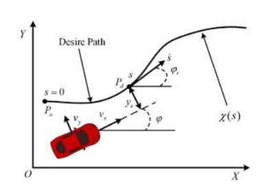
This paper presents a nonlinear robust H-infinity control strategy for improving trajectory following performance of autonomous ground electric vehicles (AGEV) with active front steering system. Since vehicle trajectory dynamics inherently influenced by various driving maneuvers and road conditions, the main objective is to deal with the trajectory following control challenges of parametric uncertainties, system nonlinearities, and external disturbance. The AGEV system dynamics and its uncertain vehicle trajectory following system are first modeled and constructed, in which parameter uncertainties related to the physical limits of tire are considered and handled, then the control-oriented vehicle trajectory following augmented system with dynamic error is developed. The resulting nonlinear robust H-infinity state-feedback controller (NHC) of vehicle trajectory-following system is finally designed by H-infinity performance index and nonlinear compensation under AGEV system requirements, and solved utilizing a set of linear matrix inequalities derived from quadratic H-infinity performance and Lyapunov stability. Simulations for double lane change and serpentine scenes are carried out to verify the effectiveness of the proposed controller with a high-fidelity, CarSim^®, full-vehicle model. It is found from the results that the proposed NHC provides improved vehicle trajectory following performance compared with the linear quadratic regulator (LQR) controller and robust H-infinity state-feedback controller (RHC).
- autonomous vehicles,
- electric vehicles,
- trajectory-following,
- robust control,
- nonlinear control
Citation: Xianjian Jin, Qikang Wang, Zeyuan Yan, Hang Yang. Nonlinear robust control of trajectory-following for autonomous ground electric vehicles with active front steering system[J]. AIMS Mathematics, 2023, 8(5): 11151-11179. doi: 10.3934/math.2023565

Related Papers:

Abstract

This paper presents a nonlinear robust H-infinity control strategy for improving trajectory following performance of autonomous ground electric vehicles (AGEV) with active front steering system. Since vehicle trajectory dynamics inherently influenced by various driving maneuvers and road conditions, the main objective is to deal with the trajectory following control challenges of parametric uncertainties, system nonlinearities, and external disturbance. The AGEV system dynamics and its uncertain vehicle trajectory following system are first modeled and constructed, in which parameter uncertainties related to the physical limits of tire are considered and handled, then the control-oriented vehicle trajectory following augmented system with dynamic error is developed. The resulting nonlinear robust H-infinity state-feedback controller (NHC) of vehicle trajectory-following system is finally designed by H-infinity performance index and nonlinear compensation under AGEV system requirements, and solved utilizing a set of linear matrix inequalities derived from quadratic H-infinity performance and Lyapunov stability. Simulations for double lane change and serpentine scenes are carried out to verify the effectiveness of the proposed controller with a high-fidelity, CarSim^®, full-vehicle model. It is found from the results that the proposed NHC provides improved vehicle trajectory following performance compared with the linear quadratic regulator (LQR) controller and robust H-infinity state-feedback controller (RHC).

References

[1]	G. Demesure, M. Defoort, A. Bekrar, D. Trentesaux, M. Djemaï , Decentralized motion planning and scheduling of AGVs in an FMS, IEEE Trans. Ind. Informat., 14 (2018), 1744–1752. https://doi.org/10.1109/TII.2017.2749520 doi: 10.1109/TII.2017.2749520
[2]	S. Riazi, K. Bengtsson, B. Lennartson, Energy optimization of large-scale AGV systems, IEEE Trans. Autom. Sci. Eng., 18 (2021), 638–649. https://doi.org/10.1109/TASE.2019.2963285 doi: 10.1109/TASE.2019.2963285
[3]	V. Digani, L. Sabattini, C. Secchi, C. Fantuzzi, Ensemble coordination approach in multi-AGV systems applied to industrial warehouses, IEEE Trans. Autom. Sci. Eng., 12 (2015), 922–934. https://doi.org/10.1109/TASE.2015.2446614 doi: 10.1109/TASE.2015.2446614
[4]	T. Wang, Y. Xu, S. Ahipasaoglu, C. Courcoubetis, Ex-post max-min fairness of generalized AGV mechanisms, IEEE Trans. Autom. Control, 62 (2017), 5275–5281. https://doi.org/10.1109/TAC.2016.2632424 doi: 10.1109/TAC.2016.2632424
[5]	S. Hoshino, J. Ota, A. Shinozaki, H. Hashimoto, Hybrid design methodology and cost-effectiveness evaluation of AGV transportation systems, IEEE Trans. Autom. Sci. Eng., 4 (2007), 360–372. https://doi.org/10.1109/TASE.2006.887162 doi: 10.1109/TASE.2006.887162
[6]	S. Lu, C. Xu, R. Zhong, An active RFID tag-enabled locating approach with multipath effect elimination in AGV, IEEE Trans. Autom. Sci. Eng., 13 (2016), 1333–1342. https://doi.org/10.1109/TASE.2016.2573595 doi: 10.1109/TASE.2016.2573595
[7]	H. Gao, J. Zhu, X. Li, Y. Kang, J. Li, H. Su, Automatic parking control of unmanned vehicle based on switching control algorithm and backstepping, IEEE /ASME Trans. Mech., 27 (2022), 1233–1243. https://doi.org/10.1109/TMECH.2020.3037215 doi: 10.1109/TMECH.2020.3037215
[8]	M. Graf Plessen, D. Bernardini, H. Esen, A. Bemporad, Spatial-based predictive control and geometric corridor planning for adaptive cruise control coupled with obstacle avoidance, IEEE Trans. Control. Syst. Technol., 26 (2018), 38–50. https://doi.org/10.1109/TCST.2017.2664722 doi: 10.1109/TCST.2017.2664722
[9]	R. Utriainen, M. Pöllänen, H. Liimatainen, The safety potential of lane keeping assistance and possible actions to improve the potential, IEEE Trans. Intell. Veh., 5 (2020), 556–564. https://doi.org/10.1109/TIV.2020.2991962 doi: 10.1109/TIV.2020.2991962
[10]	W. Li, Q. Li, S. Li, R. Li, Y. Ren, W. Wang, Indirect shared control through non-zero sum differential game for cooperative automated driving, IEEE Trans. Intell. Transp. Syst., 23 (2022), 15980–15992. https://doi.org/10.1109/TITS.2022.3146895 doi: 10.1109/TITS.2022.3146895
[11]	X. Jin, J. Wang, X. He, Z. Yan, L. Xu, C. Wei, et al., Improving vibration performance of electric vehicles based on in-wheel motor-active suspension system via robust finite frequency control, IEEE Trans. Intell. Transp. Syst., 24 (2023), 1631–1643. https://doi.org/10.1109/TITS.2022.3224609 doi: 10.1109/TITS.2022.3224609
[12]	X. Jin, J. Wang, Z. Yan, L. Xu, G. Yin, N. Chen, Robust vibration control for active suspension system of in-wheel-motor-driven electric vehicle via μ-synthesis methodology, ASME J. Dyn. Sys. Meas. Control, 144 (2022), 051007. https://doi.org/10.1115/1.4053661 doi: 10.1115/1.4053661
[13]	X. Jin, Q. Wang, Z. Yan, H. Yang, J. Wang, G. Yin, A learning-based evaluation for lane departure warning system considering driving characteristics, Proc. Inst. Mech. Eng. D-J. Aut., 2022. https://doi.org/10.1177/09544070221140973 doi: 10.1177/09544070221140973
[14]	K. Nam, H. Fujimoto, Y. Hori, Advanced motion control of electric vehicles based on robust lateral tire force control via active front steering, IEEE/ASME Trans. Mech., 19 (2014), 289–299. https://doi.org/10.1109/TMECH.2012.2233210 doi: 10.1109/TMECH.2012.2233210
[15]	H. Wang, Y. Tian, H. Xu, Neural adaptive command filtered control for cooperative path following of multiple underactuated autonomous underwater vehicles along one path, IEEE Trans. Syst, Man, Cybern. Syst., 52 (2022), 2966–2978. https://doi.org/10.1109/TSMC.2021.3062077 doi: 10.1109/TSMC.2021.3062077
[16]	Y. Wang, B. Nguyen, H. Fujimoto, Y. Hori, Multirate estimation and control of body slip angle for electric vehicles based on onboard vision system, IEEE Trans. Ind. Electron., 61 (2014), 1133–1143. https://doi.org//10.1109/TIE.2013.2271596 doi: 10.1109/TIE.2013.2271596
[17]	G. Wang, Y. Liu, S. Li, Y. Tian, N. Zhang, G. Cui, New integrated vehicle stability control of active front steering and electronic stability control considering tire force reserve capability, IEEE Trans. Veh. Technol., 70 (2021), 2181–2195. https://doi.org//10.1109/TVT.2021.3056560 doi: 10.1109/TVT.2021.3056560
[18]	J. Cho, K. Huh, Active front steering for driver's steering comfort and vehicle driving stability, Int. J. Automt. Technol., 20 (2019), 589–596. https://doi.org/10.1007/s12239-019-0056-1 doi: 10.1007/s12239-019-0056-1
[19]	P. Falcone, F. Borrelli, J. Asgari, H. Tseng, D. Hrovat, Predictive active steering control for autonomous vehicle systems. IEEE Trans. Control Syst. Technol., 15 (2007), 566–580. https://doi.org/10.1109/TCST.2007.894653 doi: 10.1109/TCST.2007.894653
[20]	T. Faulwasser, R. Findeisen, Nonlinear model predictive control for constrained output path following, IEEE Trans. Autom. Control, 61 (2016), 1026–1039. https://doi.org/10.1109/TAC.2015.2466911 doi: 10.1109/TAC.2015.2466911
[21]	P. Liljeback, I. Haugstuen, K. Pettersen, Path following control of planar snake robots using a cascaded approach, IEEE Trans. Control Syst. Technol., 20 (2012), 111–126. https://doi.org/10.1109/TCST.2011.2107516 doi: 10.1109/TCST.2011.2107516
[22]	A. Hladio, C. Nielsen, D. Wang, Path following for a class of mechanical systems, IEEE Trans. Control Syst. Technol., 21 (2013), 2380–2390. https://doi.org/10.1109/TCST.2012.2223470 doi: 10.1109/TCST.2012.2223470
[23]	S. Mobayen, Robust tracking controller for multivariable delayed systems with input saturation via composite nonlinear feedback, Nonlinear. Dyn., 76 (2014), 827–838. https://doi.org/10.1007/s11071-013-1172-5 doi: 10.1007/s11071-013-1172-5
[24]	V. Ghaffari, Optimal tuning of composite nonlinear feedback control in time-delay nonlinear systems, J. Franklin Inst., 357 (2020), 1331–1356. https://doi.org/10.1016/j.jfranklin.2019.12.024 doi: 10.1016/j.jfranklin.2019.12.024
[25]	S. Yu, X. Li, H. Chen, F. Allgöwer, Nonlinear model predictive control for path following problems, Int. J. Robust Nonlinear Control, 25 (2015), 1168–1182. https://doi.org/10.1002/rnc.3133 doi: 10.1002/rnc.3133
[26]	J. Chen, Z. Shuai, H. Zhang, W. Zhao, Path following control of autonomous four-wheel-independent-drive electric vehicles via second-order sliding mode and nonlinear disturbance observer techniques, IEEE Trans. Ind. Electron., 68 (2021), 2460–2469. https://doi.org/10.1109/TIE.2020.2973879 doi: 10.1109/TIE.2020.2973879
[27]	Z. Liu, X. Chen, Adaptive sliding mode security control for stochastic Markov jump cyber-physical nonlinear systems subject to actuator failures and randomly occurring injection attacks, IEEE Trans. Ind. Informat., 2022. https://doi.org/10.1109/TII.2022.3181274 doi: 10.1109/TII.2022.3181274
[28]	X. Zhao, Z. Liu, B. Jiang, C. Gao, Switched controller design for robotic manipulator via neural network-based sliding mode approach, IEEE Trans. Circuits Syst. II: Exp. Briefs, 70 (2022), 561–565. https://doi.org/10.1109/TCSII.2022.3169475 doi: 10.1109/TCSII.2022.3169475
[29]	B. Xu, F. Sun, Y. Pan, B. Chen, Disturbance observer based composite learning fuzzy control of nonlinear systems with unknown dead zone, IEEE Trans. Syst. Man. Cybern. Syst., 47 (2017), 1854–1862. https://doi.org/10.1109/TSMC.2016.2562502 doi: 10.1109/TSMC.2016.2562502
[30]	H. A. Hagras, A hierarchical type-2 fuzzy logic control architecture for autonomous mobile robots, IEEE Trans. Fuzzy. Syst., 12 (2004), 524–539. https://doi.org/10.1109/TFUZZ.2004.832538 doi: 10.1109/TFUZZ.2004.832538
[31]	J. Cervantes, W. Yu, S. Salazar, I. Chairez, Takagi-Sugeno dynamic neuro-fuzzy controller of uncertain nonlinear systems, IEEE Trans. Fuzzy. Syst., 25 (2017), 1601–1615. https://doi.org/10.1109/TFUZZ.2016.2612697 doi: 10.1109/TFUZZ.2016.2612697
[32]	Y. Wu, L. Wang, J. Zhang, F. Li, Path following control of autonomous ground vehicle based on nonsingular terminal sliding mode and active disturbance rejection control, IEEE Trans. Veh. Technol., 68 (2019), 6379–6390. https://doi.org/10.1109/TVT.2019.2916982 doi: 10.1109/TVT.2019.2916982
[33]	M. Islam, Y. He, An optimal preview controller for active trailer steering systems of articulated heavy vehicles, SAE Tech. Pap., 2011, 1–14. https://doi.org/10.4271/2011-01-0983
[34]	T. Ding, Y. Zhang, G. Ma, Z. Cao, X. Zhao, B. Tao, Trajectory tracking of redundantly actuated mobile robot by MPC velocity control under steering strategy constraint, Mechatronics, 84 (2022), 102779. https://doi.org/10.1016/j.mechatronics.2022.102779 doi: 10.1016/j.mechatronics.2022.102779
[35]	H. Moradi, G. Vossoughi, M. R. Movahhedy, H. Salarieh, Suppression of nonlinear regenerative chatter in milling process via robust optimal control, J. Process Control, 23 (2013), 631–648. https://doi.org/10.1016/j.jprocont.2013.02.006 doi: 10.1016/j.jprocont.2013.02.006
[36]	Y. Fu, B. Li, J. Fu, Multi-model adaptive switching control of a nonlinear system and its applications in a smelting process of fused magnesia, J. Process Control, 115 (2022), 67–76. https://doi.org/10.1016/j.jprocont.2022.04.009 doi: 10.1016/j.jprocont.2022.04.009
[37]	S. Fahmy, S. Banks, Robust H_∞ control of uncertain nonlinear dynamical systems via linear time-varying approximations, Nonlinear Anal., 63 (2005), 2315–2327. https://doi.org/10.1016/j.na.2005.03.030 doi: 10.1016/j.na.2005.03.030
[38]	G. Ju, Y. Wu, W. Sun, Adaptive output feedback asymptotic stabilization of nonholonomic systems with uncertainties, Nonlinear Anal., 71 (2009), 5106–5117. https://doi.org/10.1016/j.na.2009.03.088 doi: 10.1016/j.na.2009.03.088
[39]	E. Jafari, T. Binazadeh, Observer-based improved composite nonlinear feedback control for output tracking of time-varying references in descriptor systems with actuator saturation, ISA Trans., 91 (2019), 1–10. https://doi.org/10.1016/j.isatra.2019.01.035 doi: 10.1016/j.isatra.2019.01.035
[40]	S. Mobayen, An LMI-based robust tracker for uncertain linear systems with multiple time-varying delays using optimal composite nonlinear feedback technique, Nonlinear Dyn., 80 (2015), 917–927. https://doi.org/10.1007/s11071-015-1916-5 doi: 10.1007/s11071-015-1916-5
[41]	V. Ghaffari, S. Mobayen, D. Ud, T. Rojsiraphisal, M. T. Vu, Robust tracking composite nonlinear feedback controller design for time-delay uncertain systems in the presence of input saturation, ISA Trans., 129 (2022), 88–99. https://doi.org/10.1016/j.isatra.2022.02.029 doi: 10.1016/j.isatra.2022.02.029
[42]	X. Jin, Z. Yan, G. Yin, S. Li, C. Wei, An adaptive motion planning technique for on-road autonomous driving, IEEE Access, 9(2020), 2655–2664. https://doi.org/10.1109/ACCESS.2020.3047385 doi: 10.1109/ACCESS.2020.3047385
[43]	B. Paden, M. Čáp, S. Yong, D. Yershov, E. Frazzoli, A survey of motion planning and control techniques for self-driving urban vehicles, IEEE Trans. Intell. Veh., 1 (2016), 33–55. https://doi.org/10.1109/TIV.2016.2578706 doi: 10.1109/TIV.2016.2578706

Reader Comments

Your name:*

Email:*
© 2023 the Author(s), licensee AIMS Press. This is an open access article distributed under the terms of the Creative Commons Attribution License (http://creativecommons.org/licenses/by/4.0)