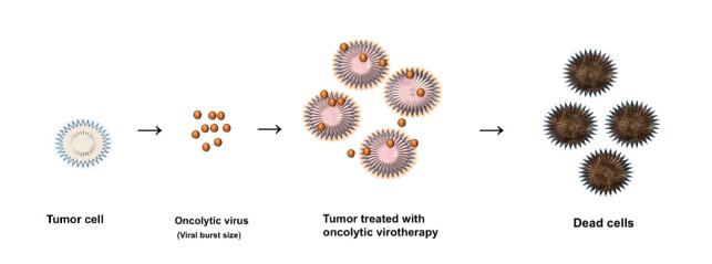
New cancer therapies, methods and protocols are needed to treat affected patients. Oncolytic viral therapy is a good suggestion for such treatment. This paper proposes a diffusive cancer model with virotherapy and an immune response. This work aims to study the aforementioned model while theoretically including positivity, boundedness and stability, as well as to find the analytical solutions. The analytical solutions are found by using the tanh-expansion method. As a result, we realized that the relative immune cell killing rate can be controlled by the viral burst size. The viral burst size is the number of viruses released from each infected cell during cell lysis. The increasing diffusion of the activated immune system leads to an increase in the uninfected cells. The presented model can be used to study the combination of immunotherapy and virotherapy.
Citation: Noufe H. Aljahdaly, Nouf A. Almushaity. A diffusive cancer model with virotherapy: Studying the immune response and its analytical simulation[J]. AIMS Mathematics, 2023, 8(5): 10905-10928. doi: 10.3934/math.2023553
New cancer therapies, methods and protocols are needed to treat affected patients. Oncolytic viral therapy is a good suggestion for such treatment. This paper proposes a diffusive cancer model with virotherapy and an immune response. This work aims to study the aforementioned model while theoretically including positivity, boundedness and stability, as well as to find the analytical solutions. The analytical solutions are found by using the tanh-expansion method. As a result, we realized that the relative immune cell killing rate can be controlled by the viral burst size. The viral burst size is the number of viruses released from each infected cell during cell lysis. The increasing diffusion of the activated immune system leads to an increase in the uninfected cells. The presented model can be used to study the combination of immunotherapy and virotherapy.

| [1] |
H. Fukuhara, Y. Ino, T. Todo, Oncolytic virus therapy: A new era of cancer treatment at dawn, Cancer Sci., 107 (2016), 1373–1379. https://doi.org/10.1111/cas.13027 doi: 10.1111/cas.13027

|
| [2] |
J. P. Tian, The replicability of oncolytic virus: defining conditions in tumor virotherapy, Math. Biosci. Eng., 8 (2011), 841. https://doi.org/10.13005/bbra/947 doi: 10.13005/bbra/947
|
| [3] |
S. Kumar, A. Kumar, B. Samet, J. F. Gómez-Aguilar, M. S. Osman, A chaos study of tumor and effector cells in fractional tumor-immune model for cancer treatment, Chaos Soliton. Fract., 141 (2020), 110321. https://doi.org/10.1016/j.chaos.2020.110321 doi: 10.1016/j.chaos.2020.110321
|
| [4] |
J. F. Gómez-Aguilar, M. G. López-López, V. M. Alvarado-Martínez, D. Baleanu, H. Khan, Chaos in a cancer model via fractional derivatives with exponential decay and mittag-leffler law, Entropy, 19 (2017), 681. https://doi.org/10.3390/e19120681 doi: 10.3390/e19120681
|
| [5] |
Z. Z. Zhang, G. Rahman, J. F. Gómez-Aguilar, J. Torres-Jiménez, Dynamical aspects of a delayed epidemic model with subdivision of susceptible population and control strategies, Chaos Soliton. Fract., 160 (2022), 112194. https://doi.org/10.1016/j.chaos.2022.112194 doi: 10.1016/j.chaos.2022.112194
|
| [6] | M. Umar, Z. Sabir, M. A. Z. Raja, J. F. Gómez-Aguilar, F. Amin, M. Shoaib, Neuro-swarm intelligent computing paradigm for nonlinear hiv infection model with CD4+ T-cells, Math. Comput. Simul., 188 (2021), 241–253. |
| [7] |
R. A. Alharbey, N. H. Aljahdaly, On fractional numerical simulation of hiv infection for CD8+ T-cells and its treatment, Plos One, 17 (2022), e0265627. https://doi.org/10.1371/journal.pone.0265627 doi: 10.1371/journal.pone.0265627
|
| [8] |
N. H. Aljahdaly R. A. Alharbey, Fractional numerical simulation of mathematical model of HIV-1 infection with stem cell therapy, AIMS Math., 6 (2021), 6715–6726. https://doi.org/10.3934/math.2021395 doi: 10.3934/math.2021395
|
| [9] | N. H. Aljahdaly, H. A. Ashi, Exponential time differencing method for studying prey-predator dynamic during mating period, Comput. Math. Method. M., 2021 (2021). |
| [10] |
D. Wodarz, Gene therapy for killing p53-negative cancer cells: Use of replicating versus nonreplicating agents, Hum. Gene Ther., 14 (2003), 153–159. https://doi.org/10.1089/104303403321070847 doi: 10.1089/104303403321070847
|
| [11] | Ž. Bajzer, T. Carr, K. Josić, S. J. Russell, D. Dingli, Modeling of cancer virotherapy with recombinant measles viruses, J. Theor. Biol., 252 (2008), 109–122. |
| [12] | G. Marelli, A. Howells, N. R. Lemoine, Y. H. Wang, Oncolytic viral therapy and the immune system: A double-edged sword against cancer, Front. Immunol., 9 (2018), 866. |
| [13] | N. L. Komarova, D. Wodarz, Targeted cancer treatment in silico, Model. Simul. Sci. Eng. Technol., Springer, 2014. |
| [14] | D. Wodarz, Viruses as antitumor weapons: Defining conditions for tumor remission, Cancer Res., 61 (2001), 3501–3507. |
| [15] |
D. Wodarz, N. Komarova, Towards predictive computational models of oncolytic virus therapy: Basis for experimental validation and model selection, Plos One, 4 (2009), e4271. https://doi.org/10.1371/journal.pone.0004271 doi: 10.1371/journal.pone.0004271
|
| [16] | T. A. Phan, J. P. Tian, The role of the innate immune system in oncolytic virotherapy, Comput. Math. Method. M., 2017 (2017). |
| [17] | N. Al-Johani, E. Simbawa, S. Al-Tuwairqi, Modeling the spatiotemporal dynamics of virotherapy and immune response as a treatment for cancer, Commun. Math. Biol. Neurosci., 2019 (2019). |
| [18] | E. Simbawa, N. Al-Johani, S. Al-Tuwairqi, Modeling the spatiotemporal dynamics of oncolytic viruses and radiotherapy as a treatment for cancer, Comput. Math. Method. M., 2020 (2020). |
| [19] | S. M. Al-Tuwairqi, N. O. Al-Johani, E. A. Simbawa, Modeling dynamics of cancer virotherapy with immune response, Adv. Differ. Equ., 2020 (2020), 1–26. |
| [20] | P. M. Ngina, R. W. Mbogo, L. S. Luboobi, et al., Mathematical modelling of in-vivo dynamics of HIV subject to the influence of the CD8+ T-cells, Appl. Math., 8 (2017), 1153. |
| [21] | L. Edelstein-Keshet, Mathematical models in biology, SIAM, 2005. |
| [22] | M. Martcheva, Analysis of complex ode epidemic models: Global stability, In An Introduction to Mathematical Epidemiology, Springer, 2015,149–181. |
| [23] | H. Jahanshahi, K. Shanazari, M. Mesrizadeh, S. Soradi-Zeid, J. F. Gómez-Aguilar, Numerical analysis of galerkin meshless method for parabolic equations of tumor angiogenesis problem, Eur. Phys. J. Plus, 135 (2020), 1–23. |
| [24] |
R. A. M. Attia, J. Tian, D. Lu, J. F. Gómez-Aguilar, M. M. A. Khater, Unstable novel and accurate soliton wave solutions of the nonlinear biological population model, Arab J. Basic Appl. Sci., 29 (2022), 19–25. https://doi.org/10.1080/25765299.2021.2024652 doi: 10.1080/25765299.2021.2024652
|
| [25] |
A. M. Wazwaz, The tanh method for traveling wave solutions of nonlinear equations, Appl. Math. Comput., 154 (2004), 713–723. https://doi.org/10.1155/S1073792804132157 doi: 10.1155/S1073792804132157
|
| [26] | I. H. Sahin, G. Askan, Z. I. Hu, E. M. O. Reilly, Immunotherapy in pancreatic ductal adenocarcinoma: An emerging entity? Ann. Oncol., 28 (2017), 2950–2961. https://doi.org/10.1093/annonc/mdx503 |
| [27] |
O. Nave, M. Sigron, A mathematical model for the treatment of melanoma with the BRAF/MEK inhibitor and Anti-PD-1, Appl. Sci., 12 (2022), 12474. https://doi.org/10.3390/app122312474 doi: 10.3390/app122312474
|
| [28] | E. Oh, J. E. Oh, J. W. Hong, Y. H. Chung, Y. Lee, K. D. Park, et al., Optimized biodegradable polymeric reservoir-mediated local and sustained co-delivery of dendritic cells and oncolytic adenovirus co-expressing IL-12 and GM-CSF for cancer immunotherapy, J. Control. Release, 259 (2017), 115–127. |
Figures(5) / Tables(1)

Noufe H. Aljahdaly, Nouf A. Almushaity. A diffusive cancer model with virotherapy: Studying the immune response and its analytical simulation[J]. AIMS Mathematics, 2023, 8(5): 10905-10928. doi: 10.3934/math.2023553


 DownLoad: