This study aims to propose and analyze a mathematical model of the competitive interaction of the pathogen-immune system. Some effects of the existence of natural delays and the addition of therapeutic proteins are considered in the model. A delay arises from the indirect response of the host body when a pathogen invades. The other comes from the maturation of immune cells to produce immune memory cells since the immune system and antigenic substances responsible for provoking the production of immune memory cells. Analytical investigations suggest several sufficient conditions for the existence of a positive steady-state solution. There is a critical pair of delays at which oscillatory behavior appears around the positive steady-state solution. Numerical simulations were carried out to describe the results of the analysis and show that the proposed model can describe the speed of pathogen eradication due to the addition of therapeutic proteins as antigenic substances.
Citation: Kasbawati, Yuliana Jao, Nur Erawaty. Dynamic study of the pathogen-immune system interaction with natural delaying effects and protein therapy[J]. AIMS Mathematics, 2022, 7(5): 7471-7488. doi: 10.3934/math.2022419
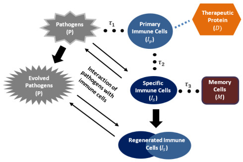
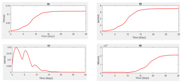
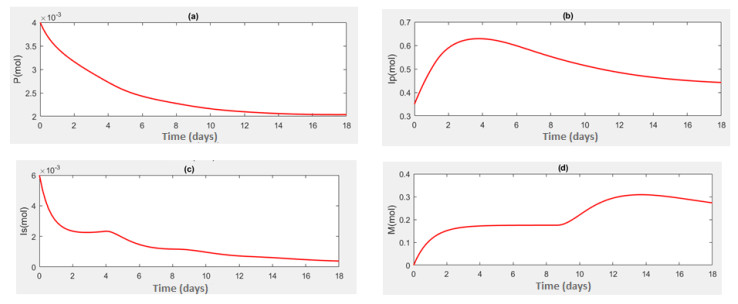
This study aims to propose and analyze a mathematical model of the competitive interaction of the pathogen-immune system. Some effects of the existence of natural delays and the addition of therapeutic proteins are considered in the model. A delay arises from the indirect response of the host body when a pathogen invades. The other comes from the maturation of immune cells to produce immune memory cells since the immune system and antigenic substances responsible for provoking the production of immune memory cells. Analytical investigations suggest several sufficient conditions for the existence of a positive steady-state solution. There is a critical pair of delays at which oscillatory behavior appears around the positive steady-state solution. Numerical simulations were carried out to describe the results of the analysis and show that the proposed model can describe the speed of pathogen eradication due to the addition of therapeutic proteins as antigenic substances.

| [1] |
D. D. Chaplin, Overview of the immune response, J. Allergy. Clin. Immun., 125 (2010), S3–S23. https://doi.org/10.1016/j.jaci.2009.12.980 doi: 10.1016/j.jaci.2009.12.980

|
| [2] | C. A. Jr. Janeway, P. Travers, M. Walport, et al., Immunobiology: The Immune System in Health and Disease. 5th edition. New York: Garland Science, 2001. |
| [3] |
C. R. Maldini, G. I. Ellis, J. L. Riley, CAR T cells for infection, autoimmunity and allotransplantation, Nat. Rev. Immunol., 18 (2018), 605–616. https://doi.org/10.1038/s41577-018-0042-2 doi: 10.1038/s41577-018-0042-2
|
| [4] |
L. B. Nicholson, The immune system, Essays Biochem., 60 (2016), 275–301. https://doi.org/10.1042/EBC20160017 doi: 10.1042/EBC20160017
|
| [5] |
J. M. Carton, W. R. Strohl, Protein therapeutics (introduction to biopharmaceuticals): Introduction to Biological and Small Molecule Drug Research and Development, Elsevier, 2013,127–159, ISBN 9780123971760, https://doi.org/10.1016/B978-0-12-397176-0.00004-2. |
| [6] | M. Lever, T. D. C. Hirata, P. Russo, H. I. Nakaya, Systems immunology, Theoretical and Applied Aspects of Systems Biology., Springer International Publishing (2018), 159–173. https://doi.org/10.1007/978-3-319-74974-7. |
| [7] |
N. Chirmule, V. Jawa, B. Mibohm, Immunogenicity to therapeutic proteins: impact on PK/PD and efficacy, AAPS J., 14 (2012), 296–302. https://doi.org/10.1208/s12248-012-9340-y doi: 10.1208/s12248-012-9340-y
|
| [8] | K. Bloem, B. Hernández-Breijo, A. Martínez-Feito, T. Rispens, Immunogenicity of therapeutic antibodies: Monitoring antidrug antibodies in a clinical context, Ther Drug Monit., 4 (2017), 327–332. https://doi.org/10.1097/FTD.0000000000000404 |
| [9] |
J. J. P. Ruixo, P. Ma, A. T. Chow, The utility of modeling and simulation approaches to evaluate immunogenicity effect on the therapeutic protein pharmacokinetics, AAPS J., 15 (2013), 172–182. https://doi.org/10.1208/s12248-012-9424-8 doi: 10.1208/s12248-012-9424-8
|
| [10] |
R. Eftimie, J. J. Gillard, D. A. Cantrell, Mathematical models for immunology: Current state of the art and future research directions, B. Math. Biol., 78 (2016), 2091–2134. https://doi.org/10.1007/s11538-016-0214-9 doi: 10.1007/s11538-016-0214-9
|
| [11] |
S. Banerjee, S. Khajanchi, S. Chaudhuri, A mathematical model to elucidate brain tumor abrogation by immunotherapy with T11 target structure, PLoS ONE, 10 (2015), e0123611, https://doi.org/10.1371/journal.pone.0123611. doi: 10.1371/journal.pone.0123611
|
| [12] |
J. Reyes-Silveyra, A. R. Mikler, Modeling immune response and its effect on infectious disease outbreak dynamic, Theor. Biol. Med. Model., 13 (2016). https://doi.org/10.1186/s12976-016-0033-6 doi: 10.1186/s12976-016-0033-6
|
| [13] |
S. Kathman, T. M. Thway, L. Zhou, S. Lee, Utility of a bayesian mathematical model to predict the impact of immunogenicity on pharmacokinetics of therapeutic proteins, AAPS J., 18 (2016), 424–431. https://doi.org/10.1208/s12248-015-9853-2 doi: 10.1208/s12248-015-9853-2
|
| [14] |
W. L. Duan, H. Fang, C. Zeng, The stability analysis of tumor-immune responses to chemotherapy system with gaussian white noises. Chaos, Soliton. Fract., 127 (2019), 96–102. https://doi.org/10.1016/j.chaos.2019.06.030. doi: 10.1016/j.chaos.2019.06.030
|
| [15] |
G. A. Bocharov, V. Volpert, B. Ludewig, A. Meyerhans, Mathematical modeling of the immune system in homeostasis, infection and disease, Front. Immunol., 10 (2020), 2944. https://doi.org/10.3389/fimmu.2019.02944 doi: 10.3389/fimmu.2019.02944
|
| [16] |
G. A. Bocharov, D. S. Grebennikov, R. S. Savinkov, Mathematical immunology: From phenomenological to multiphysics modelling, Russ. J. Numer. Anal. Mathematical M., 35 (2020), 203–213. https://doi.org/10.1515/rnam-2020-0017 doi: 10.1515/rnam-2020-0017
|
| [17] |
S. A. Alharbi, A. Z. Rambely, Dynamic behaviour and stabilisation to boost the immune system by complex interaction between tumour cells and vitamins intervention, Adv. Differ. Equ-Ny., 1 (2020), 412. https://doi.org/10.1186/s13662-020-02869-6 doi: 10.1186/s13662-020-02869-6
|
| [18] |
A. Fenton, J. Lello, M. B. Bonsall, Pathogen responses to host immunity: The impact of time delays and memory on the evolution of virulence, Proc. R. Soc. B., 273 (2006). https://doi.org/10.1098/rspb.2006.3552 doi: 10.1098/rspb.2006.3552
|
| [19] |
F. A. Rihan, D. H. A. Rahman, Delay differential model for tumour-immune dynamics with HIV infection of CD4+ T-cells, Int. J. Comput. Math., 90 (2013), 594–614, http://dx.doi.org/10.1080/00207160.2012.726354. doi: 10.1080/00207160.2012.726354
|
| [20] |
F. A. Rihan, D. H. Abdelrahman, F. Al-Maskari, F. Ibrahim, M. A. Abdeen, Delay differential model for tumour-immune response with chemoimmunotherapy and optimal control, Comput. Math. Method. M., 2014 (2014), Article ID 982978. http://dx.doi.org/10.1155/2014/982978. |
| [21] |
S. Khajanchi, S. Banerjee, Stability and bifurcation analysis of delay induced tumor immune interaction model, Appl. Math. Comput., 248 (2014), 652–671. https://doi.org/10.1016/j.amc.2014.10.009. doi: 10.1016/j.amc.2014.10.009
|
| [22] |
S. Kayan, H. Merdan, R. Yafia, S. Goktepe, Bifurcation analysis of a modified tumor-immune system interaction model involving time delay, Math. Model. Nat. Pheno., 12 (2017), 120–145. https://doi.org/10.1051/mmnp/201712508 doi: 10.1051/mmnp/201712508
|
| [23] |
F. A. Rihan, S. Lakshmanan, H. Maurer, Optimal control of tumour-immune model with time-delay and immuno-chemotherapy. Appl. Math. Comput., 353 (2019), 147–165. https://doi.org/10.1016/j.amc.2019.02.002. doi: 10.1016/j.amc.2019.02.002
|
| [24] |
J. P. Mendonça, I. Gleria, M. L. Lyra, Delay-induced bifurcations and chaos in a two-dimensional model for the immune response, Physica A, 517 (2019), 484–490. https://doi.org/10.1016/j.physa.2018.11.039 doi: 10.1016/j.physa.2018.11.039
|
| [25] |
F. Fatehi, Y. N. Kyrychko, K. B. Blyuss, Time-delayed model of autoimmune dynamics, Math. Biosci. Eng., 16 (2019), 5613–5639. https://doi.org/10.3934/mbe.2019279 doi: 10.3934/mbe.2019279
|
| [26] |
Kasbawati, Mariani, N. Erawaty, N. Aris, A mathematical study of effects of delays arising from the interaction of anti-drug antibody and therapeutic protein in the immune response system, AIMS Math., 5 (2020), 7191–7213. https://doi.org/10.3934/math.2020460 doi: 10.3934/math.2020460
|
| [27] |
P. Das, P. Das, S. Das, Effects of delayed immune-activation in the dynamics of tumor-immune interactions, Math. Model. Nat. Pheno., 15 (2020), 45. https://doi.org/10.1051/mmnp/2020001 doi: 10.1051/mmnp/2020001
|
| [28] |
Q. Tang, G. Zhang, Stability and Hopf bifurcations in a competitive tumour-immune system with intrinsic recruitment delay and chemotherapy, Math. Biosci. Eng., 18 (2021), 1941–1965. https://doi.org/10.3934/mbe.2021101 doi: 10.3934/mbe.2021101
|
| [29] |
W. L. Duan, L. Lin, Noise and delay enhanced stability in tumor-immune responses to chemotherapy system, Chaos, Soliton. Fract., 148 (2021), 111019. https://doi.org/10.1016/j.chaos.2021.111019. doi: 10.1016/j.chaos.2021.111019
|
Figures(3) / Tables(1)

Kasbawati, Yuliana Jao, Nur Erawaty. Dynamic study of the pathogen-immune system interaction with natural delaying effects and protein therapy[J]. AIMS Mathematics, 2022, 7(5): 7471-7488. doi: 10.3934/math.2022419


 DownLoad: