An intuitionistic fuzzy site selection decision framework for waste-to-energy projects from the perspective of "Not In My Backyard" risk

Yuanlu Qiao; Jingpeng Wang; Yuanlu Qiao; Jingpeng Wang

doi:10.3934/math.2023184

AIMS Mathematics

2023, Volume 8, Issue 2: 3676-3698. doi: 10.3934/math.2023184

Previous Article Next Article

Research article Special Issues

An intuitionistic fuzzy site selection decision framework for waste-to-energy projects from the perspective of "Not In My Backyard" risk

Yuanlu Qiao ^,,
Jingpeng Wang

School of Management Engineering, Qingdao University of Technology, Qingdao 266520, China

Received: 03 October 2022 Revised: 09 November 2022 Accepted: 13 November 2022 Published: 24 November 2022
MSC : 03E72, 90B50

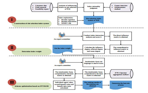
In the process of site selection for waste-to-energy (WtE) projects, the public is concerned about the impact of project construction on the surrounding environment and physical health and thus resists the construction site, leading to the emergence of "Not In My Backyard" (NIMBY) risk, which hinders the implementation of WtE projects. These risks make the ambiguity and uncertainty of scheme evaluation and decision higher. In this regard, this study constructed a WtE project site selection decision framework based on comprehensive consideration of NIMBY risk. Firstly, indicators were selected from cost perception, benefit expectation, and NIMBY risk to construct a WtE project site selection indicator system. Then, based on the "Decision Making Trial and Evaluation Laboratory" (DEMATEL) and the Intuitionistic Fuzzy Multi-criteria Optimization and Compromise Solution (IFVIKOR) method, a site selection decision framework is constructed. The system takes into account the interaction between indicators and obtains a more reasonable index weight. Meanwhile, the intuitionistic fuzzy theory is used to solve the fuzziness and uncertainty in risk assessment and decision-making. Finally, the feasibility of the siting decision system was verified through case studies. The results show that the A3 in this case was considered the best location for the project. In addition, the sensitivity analysis verifies the reliability and stability of the WtE project location decision framework.
- site selection,
- waste-to-energy project,
- NIMBY risk,
- intuitionistic fuzzy set,
- DEMATEL
Citation: Yuanlu Qiao, Jingpeng Wang. An intuitionistic fuzzy site selection decision framework for waste-to-energy projects from the perspective of 'Not In My Backyard' risk[J]. AIMS Mathematics, 2023, 8(2): 3676-3698. doi: 10.3934/math.2023184

Related Papers:

Abstract

In the process of site selection for waste-to-energy (WtE) projects, the public is concerned about the impact of project construction on the surrounding environment and physical health and thus resists the construction site, leading to the emergence of "Not In My Backyard" (NIMBY) risk, which hinders the implementation of WtE projects. These risks make the ambiguity and uncertainty of scheme evaluation and decision higher. In this regard, this study constructed a WtE project site selection decision framework based on comprehensive consideration of NIMBY risk. Firstly, indicators were selected from cost perception, benefit expectation, and NIMBY risk to construct a WtE project site selection indicator system. Then, based on the "Decision Making Trial and Evaluation Laboratory" (DEMATEL) and the Intuitionistic Fuzzy Multi-criteria Optimization and Compromise Solution (IFVIKOR) method, a site selection decision framework is constructed. The system takes into account the interaction between indicators and obtains a more reasonable index weight. Meanwhile, the intuitionistic fuzzy theory is used to solve the fuzziness and uncertainty in risk assessment and decision-making. Finally, the feasibility of the siting decision system was verified through case studies. The results show that the A3 in this case was considered the best location for the project. In addition, the sensitivity analysis verifies the reliability and stability of the WtE project location decision framework.

References

[1]	I. R. Istrate, D. Iribarren, J. L. Gálvez-Martos, J. Dufour, Review of life-cycle environmental consequences of waste-to-energy solutions on the municipal solid waste management system, Resour. Conserv. Recycl., 157 (2020), 104778. https://doi.org/10.1016/j.resconrec.2020.104778 doi: 10.1016/j.resconrec.2020.104778
[2]	Y. T. Chong, K. M. Teo, L. C. Tang, A lifecycle-based sustainability indicator framework for waste-to-energy systems and a proposed metric of sustainability, Renew. Sustain. Energy Rev., 56 (2016), 797–809. https://doi.org/10.1016/j.rser.2015.11.036 doi: 10.1016/j.rser.2015.11.036
[3]	X. G. Zhao, G. W. Jiang, A. Li. Y. Li, Technology, cost, a performance of waste-to-energy incineration industry in China, Renew. Sustain. Energy Rev., 55 (2016), 115–130. https://doi.org/10.1016/j.rser.2015.10.137
[4]	K. Ghoseiri, J. Lessan, Waste disposal site selection using an analytic hierarchal pairwise comparison and ELECTRE approaches under fuzzy environment, J. Intell. Fuzzy Syst., 26 (2014), 693–704. https://doi.org/10.3233/IFS-120760 doi: 10.3233/IFS-120760
[5]	L. Wang, X. Zhang, Bayesian analytics for estimating risk probability in PPP waste-to-energy projects, J. Manag. Eng., 34 (2018), 1–13. https://doi.org/10.1061/(asce)me.1943-5479.0000658 doi: 10.1061/(asce)me.1943-5479.0000658
[6]	Y. Wu, J. Wang, Y. Hu, Y. Ke, L. Li, An extended TODIM-PROMETHEE method for waste-to-energy plant site selection based on sustainability perspective, Energy, 156 (2018), 1–16. https://doi.org/10.1016/j.energy.2018.05.087 doi: 10.1016/j.energy.2018.05.087
[7]	B. Saveyn, On NIMBY and commuting, Int. Tax Public Financ., 20 (2013), 293–311. https://doi.org/10.1007/s10797-012-9228-x
[8]	S. Belayutham, V. A. González, T. W. Yiu, A cleaner production-pollution prevention based framework for construction site induced water pollution, J. Clean. Prod., 135 (2016), 1363–1378. https://doi.org/10.1016/j.jclepro.2016.07.003 doi: 10.1016/j.jclepro.2016.07.003
[9]	J. Song, D. Song, D. Zhang, Modeling the concession period and subsidy for BOT waste-to-energy incineration projects, J. Constr. Eng. Manag., 141 (2015). https://doi.org/10.1061/(asce)co.1943-7862.0001005
[10]	N. Komendantova, A. Battaglini, Beyond Decide-Announce-Defend (DAD) and Not-in-My-Backyard (NIMBY) models? Addressing the social and public acceptance of electric transmission lines in Germany, Energy Res. Soc. Sci., 22 (2016), 224–231. https://doi.org/10.1016/j.erss.2016.10.001 doi: 10.1016/j.erss.2016.10.001
[11]	L. Sun, D. Zhu, E. H. W. Chan, Public participation impact on environment NIMBY conflict and environmental conflict management: comparative analysis in Shanghai and Hong Kong, Land Use Policy., 58 (2016), 208–217. https://doi.org/10.1016/j.landusepol.2016.07.025 doi: 10.1016/j.landusepol.2016.07.025
[12]	M. A. Petrova, From NIMBY to acceptance: toward a novel framework-VESPA-for organizing and interpreting community concerns, Renew. Energy., 86 (2016), 1280–1294. https://doi.org/10.1016/j.renene.2015.09.047 doi: 10.1016/j.renene.2015.09.047
[13]	R. J. Johnson, M. J. Scicchitano, Don't call me NIMBY: public attitudes toward solid waste facilities, Environ. Behav., 44 (2012), 410–426. https://doi.org/10.1177/0013916511435354 doi: 10.1177/0013916511435354
[14]	D. M. McLaughlin, B. B. Cutts, Neither knowledge deficit nor NIMBY: Understanding opposition to hydraulic fracturing as a nuanced coalition in westmoreland county, Pennsylvania (USA), Environ. Manage., 62 (2018), 305–322. https://doi.org/10.1007/s00267-018-1052-3 doi: 10.1007/s00267-018-1052-3
[15]	H. Jenkins-Smith, H. Kunreuther, Mitigation and benefits measures as policy tools for siting potentially hazardous facilities: determinants of effectiveness and appropriateness, Risk Anal., 21 (2001), 371–382. https://doi.org/10.1111/0272-4332.212118 doi: 10.1111/0272-4332.212118
[16]	Y. Wu, G. Zhai, S. Li, C. Ren, S. Tsuchida, Comparative research on NIMBY risk acceptability between Chinese and Japanese college students, Environ. Monit. Assess., 186 (2014), 6683–6694. https://doi.org/10.1007/s10661-014-3882-7 doi: 10.1007/s10661-014-3882-7
[17]	P. Devine-Wright, Explaining "NIMBY" objections to a power line: the role of personal, place attachment and project-related factors, Environ. Behav., 45 (2013), 761–781. https://doi.org/10.1177/0013916512440435
[18]	A. Schwenkenbecher, What is wrong with nimbys? Renewable energy, landscape impacts and incommensurable values, Environ. Values, 26 (2017), 711–732. https://doi.org/10.3197/096327117X15046905490353 doi: 10.3197/096327117X15046905490353
[19]	E. K. Zavadskas, R. Baušys, M. Lazauskas, Sustainable assessment of alternative sites for the construction of a waste incineration plant by applying WASPAS method with single-valued neutrosophic set, Sustainability, 7 (2015), 15923–15936. https://doi.org/10.3390/su71215792 doi: 10.3390/su71215792
[20]	G. Tavares, Z. Zsigraiová, V. Semiao, Multi-criteria GIS-based siting of an incineration plant for municipal solid waste, Waste Manag., 31 (2011), 1960–1972. https://doi.org/10.1016/j.wasman.2011.04.013 doi: 10.1016/j.wasman.2011.04.013
[21]	M. Eskandari, M. Homaee, S. Mahmodi, An integrated multi criteria approach for landfill siting in a conflicting environmental, economical and socio-cultural area, Waste Manag., 32 (2012), 1528–1538. https://doi.org/10.1016/j.wasman.2012.03.014 doi: 10.1016/j.wasman.2012.03.014
[22]	M. Ekmekçioĝlu, T. Kaya, C. Kahraman, Fuzzy multicriteria disposal method and site selection for municipal solid waste, Waste Manag., 30 (2010), 1729–1736. https://doi.org/10.1016/j.wasman.2010.02.031 doi: 10.1016/j.wasman.2010.02.031
[23]	X. Pan, Y. Wang, K. S. Chin, A large-scale group decision-making method for site selection of waste to energy project under interval Type-2 fuzzy environment, Sustain. Cities Soc., 71 (2021), 103003. https://doi.org/10.1016/j.scs.2021.103003 doi: 10.1016/j.scs.2021.103003
[24]	J. Gao, X. Li, F. Guo, X. Huang, H. Men, M. Li, Site selection decision of waste-to-energy projects based on an extended cloud-TODIM method from the perspective of low-carbon, J. Clean. Prod., 303 (2021), 127036. https://doi.org/10.1016/j.jclepro.2021.127036 doi: 10.1016/j.jclepro.2021.127036
[25]	Y. Wu, L. Qin, C. Xu, S. Ji, Site selection of waste-to-energy (WtE) plant considering public satisfaction by an extended VIKOR method, Math. Probl. Eng., 2018 (2018). https://doi.org/10.1155/2018/5213504 doi: 10.1155/2018/5213504
[26]	M. Rezaei-Shouroki, A. Mostafaeipour, M. Qolipour, Prioritizing of wind farm locations for hydrogen production: a case study, Int. J. Hydrogen Energy, 42 (2017), 9500–9510. https://doi.org/10.1016/j.ijhydene.2017.02.072 doi: 10.1016/j.ijhydene.2017.02.072
[27]	M. Jahangiri, M. Rezaei, A. Mostafaeipour, A. R. Goojani, H. Saghaei, S. J. Hosseini Dehshiri, et al., Prioritization of solar electricity and hydrogen co-production stations considering PV losses and different types of solar trackers: a TOPSIS approach, Renew. Energy, 186 (2022), 889–903. https://doi.org/10.1016/j.renene.2022.01.045
[28]	M. Rezaei, K. R. Khalilpour, M. Jahangiri, Multi-criteria location identification for wind/solar based hydrogen generation: the case of capital cities of a developing country, Int. J. Hydrogen Energy, 45 (2020), 33151–33168. https://doi.org/10.1016/j.ijhydene.2020.09.138 doi: 10.1016/j.ijhydene.2020.09.138
[29]	M. Rezaei, S. A. Alharbi, A. Razmjoo, M. A. Mohamed, Accurate location planning for a wind-powered hydrogen refueling station: fuzzy VIKOR method, Int. J. Hydrogen Energy, 46 (2021), 33360–33374. https://doi.org/10.1016/j.ijhydene.2021.07.154 doi: 10.1016/j.ijhydene.2021.07.154
[30]	M. Akram, G. Ali, J. C. R. Alcantud, New decision-making hybrid model: intuitionistic fuzzy N-soft rough sets, Soft Comput., 23 (2019), 9853–9868. https://doi.org/10.1007/s00500-019-03903-w doi: 10.1007/s00500-019-03903-w
[31]	J. C. R. Alcantud, A. Z. Khameneh, A. Kilicman, Aggregation of infinite chains of intuitionistic fuzzy sets and their application to choices with temporal intuitionistic fuzzy information, Inf. Sci. Ny., 514 (2020), 106–117. https://doi.org/10.1016/j.ins.2019.12.008 doi: 10.1016/j.ins.2019.12.008
[32]	X. Zhao, X. Zhao, G. Jiang, A. Li, L. Wang, Economic analysis of waste-to-energy industry in China, Waste Manag., 48 (2016), 604–618. https://doi.org/10.1016/j.wasman.2015.10.014 doi: 10.1016/j.wasman.2015.10.014
[33]	C. Luo, Y. Ju, E. D. R. Santibanez Gonzalez, P. Dong, A. Wang, The waste-to-energy incineration plant site selection based on hesitant fuzzy linguistic best-worst method ANP and double parameters TOPSIS approach: a case study in China, Energy, 211 (2020), 118564. https://doi.org/10.1016/j.energy.2020.118564 doi: 10.1016/j.energy.2020.118564
[34]	C. Sun, X. Meng, S. Peng, Effects of waste-to-energy plants on China's urbanization: evidence from a hedonic price analysis in Shenzhen, Sustainability, 9 (2017), 1–18. https://doi.org/10.3390/su9030475 doi: 10.3390/su9030475
[35]	Y. Wu, K. Chen, B. Zeng, M. Yang, S. Geng, Cloud-based decision framework for waste-to-energy plant site selection - a case study from China, Waste Manag., 48 (2026), 593–603. https://doi.org/10.1016/j.wasman.2015.11.030 doi: 10.1016/j.wasman.2015.11.030
[36]	J. Song, D. Song, X. Zhang, Y. Sun, Risk identification for PPP waste-to-energy incineration projects in China, Energy Policy, 61 (2013), 953–962. https://doi.org/10.1016/j.enpol.2013.06.041 doi: 10.1016/j.enpol.2013.06.041
[37]	Y. Wu, J. Zhou, Y. Hu, L. Li, X. Sun, A TODIM-based investment decision framework for commercial distributed PV projects under the energy performance contracting (EPC) business model: a case in east-central China, Energies, 11 (2018). https://doi.org/10.3390/en11051210
[38]	S. Kimbrough, D. A. Vallero, R. C. Shores, W. Mitchell, Enhanced, multi criteria based site selection to measure mobile source toxic air pollutants, Transp. Res. D Transp. Environ., 16 (2011), 586–590. https://doi.org/10.1016/j.trd.2011.07.003
[39]	P. G. Savva, C. N. Costa, A. G. Charalambides, Environmental, economical and marketing aspects of the operation of a waste-to-energy plant in the Kotsiatis Landfill in Cyprus, Waste Biomass Valori., 4 (2013), 259–269. https://doi.org/10.1007/s12649-012-9148-0
[40]	I. Arbulú, J. Lozano, J. Rey-Maquieira, The challenges of Tourism to waste-to-energy public-private partnerships, Renew. Sustain. Energy Rev., 72 (2017), 916–921. https://doi.org/10.1016/j.rser.2017.01.036
[41]	I. Khan, Z. Kabir, Waste-to-energy generation technologies and the developing economies: a multi-criteria analysis for sustainability assessment, Renew. Energy, 150 (2020), 320–333. https://doi.org/10.1016/j.renene.2019.12.132 doi: 10.1016/j.renene.2019.12.132
[42]	Y. Xu, A. P. C. Chan, B. Xia, Q. K. Qian, Y. Liu, Y. Peng, Critical risk factors affecting the implementation of PPP waste-to-energy projects in China, Appl. Energy, 158 (2015), 403–411. https://doi.org/10.1016/j.apenergy.2015.08.043 doi: 10.1016/j.apenergy.2015.08.043
[43]	S. Giaccaria, V. Frontuto, Perceived health status and environmental quality in the assessment of external costs of waste disposal facilities. An empirical investigation, Waste Manag. Res., 30 (2012), 864–870. https://doi.org/10.1177/0734242X12445654 doi: 10.1177/0734242X12445654
[44]	A. Thorn, Issue definition and conflict expansion: the role of risk to human health as an issue definition strategy in an environmental conflict, Policy Sci., 51 (2018), 59–76. https://doi.org/10.1007/s11077-018-9312-x doi: 10.1007/s11077-018-9312-x
[45]	P. G. Fredriksson, The siting of hazardous waste facilities in federal systems, Environ. Resour. Econ., 15 (2000), 75–87. https://doi.org/10.1023/A:1008313612369 doi: 10.1023/A:1008313612369
[46]	Q. Yang, Y. Zhu, X. Liu, L. Fu, Q. Guo, Bayesian-based NIMBY crisis transformation path discovery for municipal solid waste incineration in China, Sustainability, 11 (2019). https://doi.org/10.3390/su11082364
[47]	A. Coi, F. Minichilli, E. Bustaffa, S. Carone, M. Santoro, F. Bianchi, et al., Risk perception and access to environmental information in four areas in Italy affected by natural or anthropogenic pollution, Environ. Int., 95 (2016), 8–15. https://doi.org/10.1016/j.envint.2016.07.009
[48]	M. L. Tseng, A causal and effect decision making model of service quality expectation using grey-fuzzy DEMATEL approach, Expert Syst. Appl., 36 (2009), 7738–7748. https://doi.org/10.1016/j.eswa.2008.09.011 doi: 10.1016/j.eswa.2008.09.011
[49]	K. T. Atanassov, Intuitionistic fuzzy sets, Fuzzy Sets Syst., 20 (1986), 87–96. https://doi.org/10.1016/S0165-0114(86)80034-3
[50]	Z. Xu, Intuitionistic fuzzy aggregation operators, IEEE Trans. Fuzzy Syst., 15 (2007), 1179–1187. https://doi.org/10.1016/j.inffus.2012.01.011 doi: 10.1016/j.inffus.2012.01.011
[51]	Z. Xu, An overview of distance and similarity measures of intuitionistic fuzzy sets, Int. J. Uncertainty, Fuzziness Knowledge-Based Syst., 16 (2008), 529–555. https://doi.org/10.1007/s10462-020-09821-w
[52]	E. Szmidt, J. Kacprzyk, Distances between intuitionistic fuzzy sets, Fuzzy Sets Syst., 114 (2000), 505–518. https://doi.org/10.1016/S0165-0114(98)00244-9 doi: 10.1016/S0165-0114(98)00244-9
[53]	Y. Wu, B. Zhang, C. Xu, L. Li, Site selection decision framework using fuzzy ANP-VIKOR for large commercial rooftop PV system based on sustainability perspective, Sustain. Cities Soc., 40 (2018), 454–470. https://doi.org/10.1016/j.scs.2018.04.024 doi: 10.1016/j.scs.2018.04.024
[54]	R. Simanaviciene, L. Ustinovichius, Sensitivity analysis for multiple criteria decision making methods: TOPSIS and SAW, Procedia Soc. Behav. Sci., 2 (2010), 7743–7744. https://doi.org/10.1016/j.sbspro.2010.05.207 doi: 10.1016/j.sbspro.2010.05.207

Reader Comments

Your name:*

Email:*
© 2023 the Author(s), licensee AIMS Press. This is an open access article distributed under the terms of the Creative Commons Attribution License (http://creativecommons.org/licenses/by/4.0)