Analyzing a SEIR-Type mathematical model of SARS-COVID-19 using piecewise fractional order operators

Nadiyah Hussain Alharthi; Mdi Begum Jeelani; Nadiyah Hussain Alharthi; Mdi Begum Jeelani

doi:10.3934/math.20231382

AIMS Mathematics

2023, Volume 8, Issue 11: 27009-27032. doi: 10.3934/math.20231382

Previous Article Next Article

Research article Special Issues

Analyzing a SEIR-Type mathematical model of SARS-COVID-19 using piecewise fractional order operators

Department of mathematics and statistics, College of Science, Imam Mohammad Ibn Saud Islamic University (IMSIU), Riyadh, Saudi Arabia

Received: 23 June 2023 Revised: 17 August 2023 Accepted: 30 August 2023 Published: 22 September 2023
MSC : 34A08, 47H08, 93A30

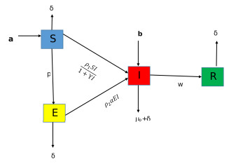
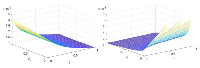
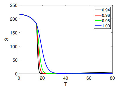
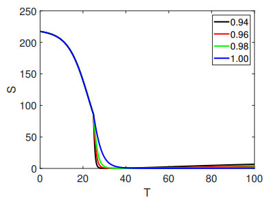
Recently, the area devoted to mathematical epidemiology has attracted much attention. Mathematical formulations have served as models for various infectious diseases. In this regard, mathematical models have also been used to study COVID-19, a threatening disease in present time. This research work is devoted to consider a SEIR (susceptible-exposed-infectious-removed) type mathematical model for investigating COVID-19 alongside a new scenario of fractional calculus. We consider piece-wise fractional order derivatives to investigate the proposed model for qualitative and computational analysis. The results related to the qualitative analysis are studied via using the tools of fixed point approach. In addition, the computational analysis is performed due to a significance of simulation to understand the transmission dynamics of COVID-19 infection in the community. In addition, a numerical scheme based on Newton's polynomials is established to simulate the approximate solutions of the proposed model by using various fractional orders. Additionally, some real data results are also shown in comparison to the numerical results.
- dynamical system,
- piecewise derivative,
- Newton polynomials,
- fractional order iterative method
Citation: Nadiyah Hussain Alharthi, Mdi Begum Jeelani. Analyzing a SEIR-Type mathematical model of SARS-COVID-19 using piecewise fractional order operators[J]. AIMS Mathematics, 2023, 8(11): 27009-27032. doi: 10.3934/math.20231382

Related Papers:

Abstract

Recently, the area devoted to mathematical epidemiology has attracted much attention. Mathematical formulations have served as models for various infectious diseases. In this regard, mathematical models have also been used to study COVID-19, a threatening disease in present time. This research work is devoted to consider a SEIR (susceptible-exposed-infectious-removed) type mathematical model for investigating COVID-19 alongside a new scenario of fractional calculus. We consider piece-wise fractional order derivatives to investigate the proposed model for qualitative and computational analysis. The results related to the qualitative analysis are studied via using the tools of fixed point approach. In addition, the computational analysis is performed due to a significance of simulation to understand the transmission dynamics of COVID-19 infection in the community. In addition, a numerical scheme based on Newton's polynomials is established to simulate the approximate solutions of the proposed model by using various fractional orders. Additionally, some real data results are also shown in comparison to the numerical results.

References

[1]	World Health Organization (WHO), Naming the coronavirus disease (COVID-19) and the virus that causes it, 2020.
[2]	D. S. Hui, E. I Azhar, T. A. Madani, F. Ntoumi, R. Kock, O. Dar, et al., The continuing 2019-nCoV epidemic threat of novel coronaviruses to global health-The latest 2019 novel coronavirus outbreak in Wuhan, China, Int. J. Infect. Dis., 91 (2020) 264–266. https://doi.org/10.1016/j.ijid.2020.01.009 doi: 10.1016/j.ijid.2020.01.009
[3]	S. Zhao, Q. Lin, J. Ran, S. S. Musa, G. Yang, W. Wang, et. al, Preliminary estimation of the basic reproduction number of novel coronavirus (2019-nCoV) in China, Int. J. Infect. Dis., 92 (2020), 214–217. https://doi.org/10.1016/j.ijid.2020.01.050 doi: 10.1016/j.ijid.2020.01.050
[4]	S. Zhao, S. S. Musa, Q. Lin, J. Ran, G. Yang, W. Wang, et al., Estimating the unreported number of novel coronavirus (2019-nCoV) cases in China in the first half of January 2020: A data-driven modelling analysis of the early outbreak, J. Clin. Med., 9 (2020), 388. https://doi.org/10.3390/jcm9020388 doi: 10.3390/jcm9020388
[5]	A. Parasher, COVID-19: Current understanding of its pathophysiology, clinical presentation and treatment, Postgrad. Med. J., 97 (2021), 312–320. https://doi.org10.1136/postgradmedj-2020-138577 doi: 10.1136/postgradmedj-2020-138577
[6]	W. M. El-Sadr, A. Vasan, A. El-Mohandes, Facing the new Covid-19 reality, N. Engl. J. Med., 388 (2023), 385–387. https://doi.org/10.1056/NEJMp2213920 doi: 10.1056/NEJMp2213920
[7]	I. Nesteruk, Statistics based predictions of coronavirus 2019-nCoV spreading in mainland China, 2020. MedRxiv.
[8]	K. Shah, R. U. Din, W. Deebani, P. Kumam, Z. Shah, On nonlinear classical and fractional order dynamical system addressing COVID-19, Results Phys., 24 (2021), 104069. https://doi.org/10.1016/j.rinp.2021.104069 doi: 10.1016/j.rinp.2021.104069
[9]	A. J. Lotka, Contribution to the theory of periodic reactions, J. Phys. Chem., 14 (2002), 271–274. https://doi.org/10.1021/j150111a004 doi: 10.1021/j150111a004
[10]	N. S. Goel, S. C. Maitra, E. W. Montroll, On the Volterra and other nonlinear models of interacting populations, Rev. Mod. phys., 43 (1971), 231–276. https://doi.org/10.1103/RevModPhys.43.231 doi: 10.1103/RevModPhys.43.231
[11]	M. M. Khalsaraei, An improvement on the positivity results for 2-stage explicit Runge-Kutta methods, J. Comput. Appl. Math., 235 (2010), 137–143. https://doi.org/10.1016/j.cam.2010.05.020 doi: 10.1016/j.cam.2010.05.020
[12]	P. Zhou, X. L. Yang, X. G. Wang, B. Hu, L. Zhang, W. Zhang, et al., A pneumonia outbreak associated with a new coronavirus of probable bat origin, Nature, 579 (2020), 270–273. https://doi.org/10.1038/s41586-020-2012-7 doi: 10.1038/s41586-020-2012-7
[13]	Q. Li, X. Guan, P. Wu, X. Wang, L. Zhou, Y. Tong, et al., Early transmission dynamics in Wuhan, China, of novel coronavirus infected pneumonia, N. Engl. J. Med., 382 (2020), 1199–1207. https://doi.org/10.1056/NEJMoa2001316 doi: 10.1056/NEJMoa2001316
[14]	I. I. Bogoch, A. Watts, A. Thomas-Bachli, C. Huber, M. U. G. Kraemer, K. Khan, Pneumonia of unknown aetiology in Wuhan, China: Potential for international spread via commercial air travel, J. Travel Med., 27 (2020), taaa008. https://doi.org/10.1093/jtm/taaa008 doi: 10.1093/jtm/taaa008
[15]	A. B. Gumel, S. Ruan, T. Day, J. Watmough, F. Brauer, P van den Driessche, et al., Modelling strategies for controlling SARS out breaks, Proc. Biol. Sci., 271 (2004), 2223–2232. https://doi.org/10.1098/rspb.2004.2800 doi: 10.1098/rspb.2004.2800
[16]	R. Kahn, I. Holmdahl, S. Reddy, J. Jernigan, M. J. Mina, R. B. Slayton, Mathematical modeling to inform vaccination strategies and testing approaches for coronavirus disease 2019 (COVID-19) in nursing homes, Clin. Infect. Dis., 74 (2022), 597–603. https://doi.org/10.1093/cid/ciab517 doi: 10.1093/cid/ciab517
[17]	J. Mondal, S. Khajanchi, Mathematical modeling and optimal intervention strategies of the COVID-19 outbreak, Nonlinear Dyn., 2022 (2022), 177–202. https://doi.org/10.1007/s11071-022-07235-7 doi: 10.1007/s11071-022-07235-7
[18]	A. I. Abioye, O. J. Peter, H. A. Ogunseye, F. A. Oguntolu, T. A. Ayoola, A. O. Oladapo, A fractional-order mathematical model for malaria and COVID-19 co-infection dynamics. Healthc. Anal., 4 (2023), 100210. https://doi.org/10.1016/j.health.2023.100210 doi: 10.1016/j.health.2023.100210
[19]	J. T. Wu, K. Leung, G. M. Leung, Nowcasting and forecasting the potential domestic and international spread of the 2019-nCoV outbreak originating in Wuhan, China: A modelling study, Lancet, 395 (2020), 689–697. https://doi.org/10.1016/S0140-6736(20)30260-9 doi: 10.1016/S0140-6736(20)30260-9
[20]	J. T. Machado, V. Kiryakova, F. Mainardi, Recent history of fractional calculus, Commun. Nonlinear Sci. Numer. Simul., 16 (2011), 1140–1153. https://doi.org/10.1016/j.cnsns.2010.05.027 doi: 10.1016/j.cnsns.2010.05.027
[21]	F. C. Meral, T. J. Royston, R. Magin, Fractional calculus in viscoelasticity: An experimental study, Commun. Nonlinear Sci. Numer. Simul., 15 (2010), 939–945. https://doi.org/10.1016/j.cnsns.2009.05.004 doi: 10.1016/j.cnsns.2009.05.004
[22]	R. L. Magin, Fractional calculus in bioengineering, Crit. Rev. Biomed. Eng., 32 (2004), 1–104. https://doi.org/10.1615/critrevbiomedeng.v32.i1.10 doi: 10.1615/critrevbiomedeng.v32.i1.10
[23]	M. Dalir, M. Bashour, Applications of fractional calculus, Appl. Math. Sci., 4 (2010), 1021–1032.
[24]	R. L. Magin, Fractional calculus in bioengineering, Redding: Begell House, 2006.
[25]	Y. A. Rossikhin, M. V. Shitikova, Applications of fractional calculus to dynamic problems of linear and nonlinear hereditary mechanics of solids, Appl. Mech. Rev., 50 (1997), 15–67. https://doi.org/10.1115/1.3101682 doi: 10.1115/1.3101682
[26]	R. Gorenflo, F. Mainardi, Fractional calculus. In: Fractals and fractional calculus in continuum mechanics, Vienna: Springer, 1997. https://doi.org/10.1007/978-3-7091-2664-6
[27]	E. Addai, A. Adeniji, O. J. Peter, J. O Agbaje, K. Oshinubi, Dynamics of age-structure smoking models with government intervention coverage under fractal-fractional order derivatives, Fractal Fract., 7 (2023), 370. https://doi.org/10.3390/fractalfract7050370 doi: 10.3390/fractalfract7050370
[28]	M. Shimizu, W. Zhang, Fractional calculus approach to dynamic problems of viscoelastic materials. JSME Int. J. Ser. C Mech. Syst. Mach. Elem. Manuf., 42 (1999), 825–837. https://doi.org/10.1299/jsmec.42.825 doi: 10.1299/jsmec.42.825
[29]	F. Mainardi, An historical perspective on fractional calculus in linear viscoelasticity, Fract. Calc. Appl. Anal., 15 (2012), 712–717. https://doi.org/10.2478/s13540-012-0048-6 doi: 10.2478/s13540-012-0048-6
[30]	Z. Dai, Y. Peng, H. A. Mansy, R. H. Sandler, T. J Royston, A model of lung parenchyma stress relaxation using fractional viscoelasticity, Med. Eng. Phys., 37 (2015), 752–758. https://doi.org/10.1016/j.medengphy.2015.05.003 doi: 10.1016/j.medengphy.2015.05.003
[31]	M. M. Amirian, Y. Jamali, The concepts and applications of fractional order differential calculus in modeling of viscoelastic systems: A primer, Crit. Rev. Biomed. Eng., 47 (2019), 249–276. https://doi.org/10.1615/CritRevBiomedEng.2018028368 doi: 10.1615/CritRevBiomedEng.2018028368
[32]	H. Khan, J. F. Gómez-Aguilar, A. Alkhazzan, A. Khan, A fractional order HIV-TB coinfection model with nonsingular Mittag-Leffler law, Math. Method. Appl. Sci., 43 (2020), 3786–3806. https://doi.org/10.1002/mma.6155 doi: 10.1002/mma.6155
[33]	C. Celauro, C. Fecarotti, A. Pirrotta, A. C. Collop, Experimental validation of a fractional model for creep/recovery testing of asphalt mixtures, Constr. Build. Mater., 36 (2012), 458–466. https://doi.org/10.1016/j.conbuildmat.2012.04.028 doi: 10.1016/j.conbuildmat.2012.04.028
[34]	G. C. Wu, M. Luo, L. L. Huang, S. Banerjee, Short memory fractional differential equations for new memristor and neural network design, Nonlinear Dyn., 100 (2020), 3611–3623. https://doi.org/10.1007/s11071-020-05572-z doi: 10.1007/s11071-020-05572-z
[35]	A. Atangana, D. Baleanu, New fractional derivatives with non-local and non-singular kernel, 2016. arXiv: 1602.03408.
[36]	E. F. D. Goufo, Application of the Caputo-Fabrizio fractional derivative without singular kernel to Korteweg-de Vries-Burgers equation, Math. Model. Anal., 21 (2016), 188–198. https://doi.org/10.3846/13926292.2016.1145607 doi: 10.3846/13926292.2016.1145607
[37]	E. F. D. Goufo, A biomathematical view on the fractional dynamics of cellulose degradation, Fract. Calc. Appl. Anal., 18 (2015), 554–564. https://doi.org/10.1515/fca-2015-0034 doi: 10.1515/fca-2015-0034
[38]	M. B. Jeelani, Stability and computational analysis of COVID-19 using a higher order galerkin time discretization scheme, Adv. Appl. Stat., 86 (2023), 167–206. https://doi.org/10.17654/0972361723022 doi: 10.17654/0972361723022
[39]	A. Al Elaiw, F. Hafeez, M. B. Jeelani, M. Awadalla, K. Abuasbeh, Existence and uniqueness results for mixed derivative involving fractional operators, AIMS Mathematics, 8 (2023), 7377–7393. https://doi.org/10.3934/math.2023371 doi: 10.3934/math.2023371
[40]	S. K. Kabunga, E. F. D. Goufo, V. H. Tuong. Analysis and simulation of a mathematical model of tuberculosis transmission in democratic Republic of the Congo, Adv. Differ. Equ., 2020 (2020), 642. https://doi.org/10.1186/s13662-020-03091-0 doi: 10.1186/s13662-020-03091-0
[41]	A. Atangana, S. I. Araz, Mathematical model of COVID-19 spread in Turkey and South Africa: Theory, methods and applications, Adv. Differ. Equ., 2020 (2020), 659. https://doi.org/10.1186/s13662-020-03095-w doi: 10.1186/s13662-020-03095-w
[42]	A. Atangana, S. I. Araz, New concept in calculus: Piecewise differential and integral operators, Chaos Soliton. Fract., 145 (2021), 110638. https://doi.org/10.1016/j.chaos.2020.110638 doi: 10.1016/j.chaos.2020.110638
[43]	M. A. Khan, A. Atangana, Modeling the dynamics of novel coronavirus (2019-nCov) with fractional derivative, Alex. Eng. J., 59 (2020), 2379–2389. https://doi.org/10.1016/j.aej.2020.02.033 doi: 10.1016/j.aej.2020.02.033
[44]	M. A. Khan, A. Atangana, E. Alzahrani, Fatmawati, The dynamics of COVID-19 with quarantined and isolation, Adv. Differ. Equ., 2020 (2020), 425. https://doi.org/10.1186/s13662-020-02882-9 doi: 10.1186/s13662-020-02882-9
[45]	O. Dyer, Covid-19: China stops counting cases as models predict a million or more deaths, BMJ, 380 (2023), 2. https://doi.org/10.1136/bmj.p2 doi: 10.1136/bmj.p2
[46]	A. Moumen, R. Shafqat, A. Alsinai, H. Boulares, M. Cancan, M. B. Jeelani, Analysis of fractional stochastic evolution equations by using Hilfer derivative of finite approximate controllability, AIMS Mathematics, 8 (2023), 16094–16114. https://doi.org/10.3934/math.2023821 doi: 10.3934/math.2023821
[47]	A. Zeb, A. Atangana, Z. A. Khan, S. Djillali, A robust study of a piecewise fractional order COVID-19 mathematical model, Alex. Eng. J., 61 (2022), 5649–5665. https://doi.org/10.1016/j.aej.2021.11.039 doi: 10.1016/j.aej.2021.11.039
[48]	C. Y. Li, J. Yin, A pedestrian-based model for simulating COVID-19 transmission on college campus, Transportmetrica A, 19 (2023), 2005182. https://doi.org/10.1080/23249935.2021.2005182 doi: 10.1080/23249935.2021.2005182
[49]	M. S. Arshad, D. Baleanu, M. B. Riaz, M. Abbas, A novel 2-stage fractional Runge-Kutta method for a time fractional logistic growth model, Discrete Dyn. Nat. Soc., 2020 (2020), 1020472. https://doi.org/10.1155/2020/1020472 doi: 10.1155/2020/1020472
[50]	F. Liu, K. Burrage, Novel techniques in parameter estimation for fractional dynamical models arising from biological systems, Comput. Math. Appl., 62 (2011), 822–833. https://doi.org/10.1016/j.camwa.2011.03.002 doi: 10.1016/j.camwa.2011.03.002
[51]	M. T. Hoang, O. F. Egbelowo, Dynamics of a fractional-order hepatitis B epidemic model and its solutions by nonstandard numerical schemes, In: Mathematical Modelling and Analysis of Infectious Diseases, Springer, Cham, 302 (2020), 127–153. https://doi.org/10.1007/978-3-030-49896-2_5
[52]	Z. J. Fu, Z. C. Tang, H. T. Zhao, P. W. Li, T. Rabczuk, Numerical solutions of the coupled unsteady nonlinear convection-diffusion equations based on generalized finite difference method, Eur. Phys. J. Plus, 134 (2019), 272. https://doi.org/10.1140/epjp/i2019-12786-7 doi: 10.1140/epjp/i2019-12786-7
[53]	B. Wang, L. Li, Y. Wang, An efficient nonstandard finite difference scheme for chaotic fractional-order Chen system, IEEE Access, 8 (2020), 98410–98421. https://doi.org/10.1109/ACCESS.2020.2996271 doi: 10.1109/ACCESS.2020.2996271
[54]	A. J. Arenas, G. González-Parra, B. M. Chen-Charpentier, Construction of nonstandard finite difference schemes for the SI and SIR epidemic models of fractional order, Math. Comput. Simulat., 121 (2016), 48–63. https://doi.org/10.1016/j.matcom.2015.09.001 doi: 10.1016/j.matcom.2015.09.001
[55]	R. Lewandowski, Z. Pawlak, Dynamic analysis of frames with viscoelastic dampers modelled by rheological models with fractional derivatives, J. Sound Vib., 330 (2011), 923–936. https://doi.org/10.1016/j.jsv.2010.09.017 doi: 10.1016/j.jsv.2010.09.017
[56]	Pakistan population (LIVE), Available from: https://www.worldometers.info/world-population/pakistan-population/.
[57]	Pakistan COVID-19 corona tracker, Available from: https://www.coronatracker.com/country/pakistan/.
[58]	Current information about COVID-19 in Pakistan, Available from: https://www.worldometers.info/.
[59]	K. Shah, T. Abdeljawad, R. Ud Din, To study the transmission dynamic of SARS-CoV-2 using nonlinear saturated incidence rate, Physica A, 604 (2022), 127915. https://doi.org/10.1016/j.physa.2022.127915 doi: 10.1016/j.physa.2022.127915
[60]	R. Ouncharoen, K. Shah, R. Ud Din, T. Abdeljawad, A. Ahmadian, S. Salahshour, et al., Study of integer and fractional order COVID-19 mathematical model, Fractals, 31 (2023), 2340046. https://doi.org/10.1142/S0218348X23400467 doi: 10.1142/S0218348X23400467

Reader Comments

Your name:*

Email:*
© 2023 the Author(s), licensee AIMS Press. This is an open access article distributed under the terms of the Creative Commons Attribution License (http://creativecommons.org/licenses/by/4.0)