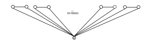
Loading [MathJax]/jax/output/SVG/jax.js
Research article Special Issues

Unbalanced signed graphs with eigenvalue properties

  • Received: 29 May 2023 Revised: 24 July 2023 Accepted: 31 July 2023 Published: 23 August 2023
  • MSC : 05C09, 05C90

  • For a signature function Ψ:E(H){±1} with underlying graph H, a signed graph (S.G) ˆH=(H,Ψ) is a graph in which edges are assigned the signs using the signature function Ψ. An S.G ˆH is said to fulfill the symmetric eigenvalue property if for every eigenvalue ˆh(ˆH) of ˆH, ˆh(ˆH) is also an eigenvalue of ˆH. A non singular S.G ˆH is said to fulfill the property (SR) if for every eigenvalue ˆh(ˆH) of ˆH, its reciprocal is also an eigenvalue of ˆH (with multiplicity as that of ˆh(ˆH)). A non singular S.G ˆH is said to fulfill the property (SR) if for every eigenvalue ˆh(ˆH) of ˆH, its negative reciprocal is also an eigenvalue of ˆH (with multiplicity as that of ˆh(ˆH)). In this article, non bipartite unbalanced S.Gs ˆC(m,1)3 and ˆC(m,2)5, where m is even positive integer have been constructed and it has been shown that these graphs fulfill the symmetric eigenvalue property, the S.Gs ˆC(m,1)3 also fulfill the properties (SR) and (SR), whereas the S.Gs ˆC(m,2)5 are close to fulfill the properties (SR) and (SR).

    Citation: Rashad Ismail, Saira Hameed, Uzma Ahmad, Khadija Majeed, Muhammad Javaid. Unbalanced signed graphs with eigenvalue properties[J]. AIMS Mathematics, 2023, 8(10): 24751-24763. doi: 10.3934/math.20231262

    Related Papers:

    [1] Guocheng Zhu, Zhining Wang, Xiaopeng Yang . On the minimal solution for max-product fuzzy relation inequalities. AIMS Mathematics, 2024, 9(11): 30667-30685. doi: 10.3934/math.20241481
    [2] Dong Pan, Huizhen Qu . Finite-time boundary synchronization of space-time discretized stochastic fuzzy genetic regulatory networks with time delays. AIMS Mathematics, 2025, 10(2): 2163-2190. doi: 10.3934/math.2025101
    [3] Ting Xie, Dapeng Li . On the stability of projected dynamical system for generalized variational inequality with hesitant fuzzy relation. AIMS Mathematics, 2020, 5(6): 7107-7121. doi: 10.3934/math.2020455
    [4] Helena Myšková, Ján Plavka . Optimizing the max-min function with a constraint on a two-sided linear system. AIMS Mathematics, 2024, 9(4): 7791-7809. doi: 10.3934/math.2024378
    [5] Ebrahim. A. Youness, Abd El-Monem. A. Megahed, Elsayed. E. Eladdad, Hanem. F. A. Madkour . Min-max differential game with partial differential equation. AIMS Mathematics, 2022, 7(8): 13777-13789. doi: 10.3934/math.2022759
    [6] Taixiang Sun, Guangwang Su, Bin Qin, Caihong Han . Global behavior of a max-type system of difference equations of the second order with four variables and period-two parameters. AIMS Mathematics, 2023, 8(10): 23941-23952. doi: 10.3934/math.20231220
    [7] Shahzaib Ashraf, Muhammad Shakir Chohan, Sameh Askar, Noman Jabbar . q-Rung Orthopair fuzzy time series forecasting technique: Prediction based decision making. AIMS Mathematics, 2024, 9(3): 5633-5660. doi: 10.3934/math.2024272
    [8] Sana Shahab, Mohd Anjum, Ashit Kumar Dutta, Shabir Ahmad . Gamified approach towards optimizing supplier selection through Pythagorean Fuzzy soft-max aggregation operators for healthcare applications. AIMS Mathematics, 2024, 9(3): 6738-6771. doi: 10.3934/math.2024329
    [9] Shahzaib Ashraf, Harish Garg, Muneeba Kousar, Sameh Askar, Shahid Abbas . Simulator selection based on complex probabilistic hesitant fuzzy soft structure using multi-parameters group decision-making. AIMS Mathematics, 2023, 8(8): 17765-17802. doi: 10.3934/math.2023907
    [10] Muhammad Bilal Khan, Muhammad Aslam Noor, Thabet Abdeljawad, Bahaaeldin Abdalla, Ali Althobaiti . Some fuzzy-interval integral inequalities for harmonically convex fuzzy-interval-valued functions. AIMS Mathematics, 2022, 7(1): 349-370. doi: 10.3934/math.2022024
  • For a signature function Ψ:E(H){±1} with underlying graph H, a signed graph (S.G) ˆH=(H,Ψ) is a graph in which edges are assigned the signs using the signature function Ψ. An S.G ˆH is said to fulfill the symmetric eigenvalue property if for every eigenvalue ˆh(ˆH) of ˆH, ˆh(ˆH) is also an eigenvalue of ˆH. A non singular S.G ˆH is said to fulfill the property (SR) if for every eigenvalue ˆh(ˆH) of ˆH, its reciprocal is also an eigenvalue of ˆH (with multiplicity as that of ˆh(ˆH)). A non singular S.G ˆH is said to fulfill the property (SR) if for every eigenvalue ˆh(ˆH) of ˆH, its negative reciprocal is also an eigenvalue of ˆH (with multiplicity as that of ˆh(ˆH)). In this article, non bipartite unbalanced S.Gs ˆC(m,1)3 and ˆC(m,2)5, where m is even positive integer have been constructed and it has been shown that these graphs fulfill the symmetric eigenvalue property, the S.Gs ˆC(m,1)3 also fulfill the properties (SR) and (SR), whereas the S.Gs ˆC(m,2)5 are close to fulfill the properties (SR) and (SR).


    In recent years, the addition-min fuzzy relation inequality (FRI) was first introduced in [1,2] for describing the flow constraints in the peer-to-peer (P2P) network system. Since the minimal solutions play a key role in constructing the complete solution set for the addition-min FRIs [3,4,5], Li et al. [1] proposed a feasible approach to find some specific minimal solutions. However, as shown in [2], the addition-min FRIs usually have an infinite number of minimal solutions, and it is difficult to determine all the minimal solutions. To obtain specific minimal solutions, various approaches have been developed. In [6], the lexicographic minimum solution was defined and studied. An effective resolution algorithm and some illustrative numerical examples were provided. The concept of the lexicographic minimum solution was also extended to random-term-absent addition-min FRIs [7]. It can be formally proven that any lexicography minimum solution should also be a minimal solution in the addition-min FRI system. In [8], Li et al. investigated another kind of minimal solution for addition-min FRIs. The authors attempted to find a minimal solution that was less than or equal to a given solution [8]. Moreover, to obtain specific minimal solutions, solving an optimization problem is also an effective approach. For instance, the optimization problem with a linear objective function was studied in [9,10], with addition-min FRIs constraints. Considering the fairness among the terminals in the P2P network system, Yang et al. [11] and Chiu et al. [12] further investigated fuzzy relation minimax programming with addition-min composition. However, it was shown that its optimal solutions were usually nonunique. Thus, Wu et al. [13] and Yang et al. [14] further searched for the minimal optimal solutions. By adding some weighted factors to the terminals, the corresponding fuzzy relation weighted minimax programming was also investigated [15,16,17].

    In references [1,2,3,4,5,6,7,8,9,10,11,12,13,14,15,16,17], addition-min FRIs were introduced to investigate the P2P network system. As noted in [18,19,20,21], by applying the addition-min FRIs to model the P2P network system, the authors considered the total download speed of each terminal and downloaded its requested data from other terminals. However, it was also indicated in [18,19,20,21] that, in some cases, the highest download speed should be considered. Next, we describe the requirements of the highest download speed for the terminals in a P2P network system. Similarly, it is assumed that there are n terminals in the system, represented by T1,T2,,Tn (see Figure 1). After accepting the downloading request from other terminals, we suppose that terminal Tj transmits its local file to any other terminal at quality level tj. If the bandwidth between Ti and Tj (exactly from Tj to Ti) is aij (see Figure 2), then the actual download traffic of Ti from Tj is aijtj.

    Figure 1.  The P2P (Peer-to-Peer) network system.
    Figure 2.  The bandwidths between Ti and the other terminals.

    Considering the total download traffic of each terminal, the P2P network system can be modeled by the addition-min FRIs. However, in some cases, the specific file should be downloaded from a single terminal. In such cases, Ti downloads its requested file from the terminal with the highest download traffic, i.e., ai1t1ai2t2aintn. Let us suppose that the requirement of the highest download traffic of Ti is no less than bi, i=1,2,,m. Then the requirements of all the terminals in a P2P network system should be modeled by the following max-min FRIs:

    ai1t1ai2t2aintnbi,i=1,2,,m. (1.1)

    Moreover, if the requirement of each terminal for the highest download speed has both an upper bound and a lower bound, then the corresponding max-min FRIs should be further written as

    biai1t1ai2t2aintndi,i=1,2,,m. (1.2)

    For inconsistent system (1.1), Yang established an evaluation model for a given vector, based on which the approximate solution was defined and investigated [22]. For the consistent system (1.1), Zhong et al. [23] focused on the lexicographic minimum solution. Xiao et al. investigated the evaluation and derived a classification of system solutions (1.1) [24]. A resolution algorithm was developed with an illustrative example. Moreover, the lexicographic minimum solution was also introduced for the above system (1.2) [25]. Then considering the stability of the P2P network system, Chen et al. [26] defined the concept of interval solutions for system (1.2). The authors proposed an effective algorithm to find the so-called widest interval solution of system (1.2) in [26].

    As mentioned above, with the constraint system of addition-min FRIs, weighted minimax programming, or even minimax programming as its specific form, has been studied, providing some efficient resolution algorithms [11,12,13,14,15,16,17]. However, when considering the highest download speed, the relevant weighted minimax programming has not been studied for the corresponding max-min system (1.2). Consequently, we focus on such an optimization problem in this work. The formulistic form of the weighted minimax programming subject to system (1.2) is

    minz(t)=c1t1c2t2cntn,s.t.{biai1t1ai2t2aintndi,i=1,2,,m. (1.3)

    As shown in [11,12,13,14,15,16,17], in system (1.2) or problem (1.3), tj (measure: Mbps) represents the quality level on which the jth terminal shares (sends out) its local resources with the other terminals. To decrease network congestion, system managers usually try to minimize the values of t1,t2,,tn. However, in most cases, these values cannot be minimized simultaneously. Instead of minimizing all these variables, minimizing a specific function with the variables t1,t2,,tn is much more realistic. For instance, in problem (1.3), we adopt the weighted minimax function. In such a weighted minimax function in (1.3), the parameter cj represents the weighted factor of the jth terminal in the P2P network system. In this work, we design several effective algorithms for identifying the optimal solution.

    In summary, the innovations and contributions of this work can be summarized as follows:

    (ⅰ) Instead of the total download traffic of the terminal, we consider the highest download traffic. Consequently, the corresponding max-min FRIs are employed.

    (ⅱ) To decrease network congestion in the P2P network system, we consider a given weighted factor for each terminal. Moreover, we further establish a relevant weighted minimax programming problem with max-min FRI constraints.

    (ⅲ) To solve our established weighted minimax optimization model, we propose the so-called single-constraint programming approach for identifying the optimal solution.

    The following content is organized as follows. In Section 2, we describe some foundational concepts and results on max-min FRIs, i.e., system (1.2). Our major results are presented in Section 3. In this section, we introduce the single-constraint programming (SCP) approach for addressing our studied problem (1.3). The original problem (1.3) is separated into several subproblems and solved. Moreover, our proposed approach is a step-by-step SCP-based algorithm. In Section 4, a detailed numerical example is provided to demonstrate the SCP-based algorithm. In Section 5, we compare our problem and the proposed method to the existing ones. Section 6 provides a simple conclusion.

    In this section, we provide some foundational results on the max-min fuzzy relation inequalities, i.e., system (1.2). These existing results are helpful for the resolution of problem (1.3).

    Let us denote

    A=(aij)m×n,t=(t1,,tn),b=(b1,,bm),d=(d1,,dm).

    Then we represent system (1.2) as

    bAtd. (2.1)

    Moreover, the solution set of system (1.2) is indeed

    TA,b,d={t[0,1]n|bAtd}.

    For convenience, we let

    I={1,2,,m},J={1,2,,n}.

    Definition 1 (Consistent; Maximum solution [25]) System (1.2) is said to be consistent when its solution set is nonempty, i.e., TA,b,d; otherwise, system (1.2) is inconsistent. When system (1.2) is consistent and there exists a solution ¯tTA,b,d such that ¯tt for any tTA,b,d, then we say ¯t is the maximum solution of (1.2).

    In system (1.2), we construct the vector ˆt=(ˆt1,ˆt2,,ˆtn) as follows:

    ˆtj={iIjdi,ifIj,1,ifIj=, (2.2)

    where Ij={iI|aij>di}, jJ. The vector ˆt is important to determine whether system (1.2) is consistent.

    Proposition 1. [25] Let tTA,b,d be a solution of system (1.2), and the vector ˆt is defined by (2.2). Then, we have tˆt.

    Theorem 1. [25] System (1.2) is consistent, i.e., TA,b,d, if and only if ˆtTA,b,d.

    According to Proposition 1 and Theorem 1, we know that when TA,b,d, ˆt should be the unique maximum solution of system (1.2). The potential maximum solution ˆt can be used to check the consistency of (1.2).

    Definition 2. (Minimal solution [25]) Let (1.2) be consistent and ˇtTA,b,d. We say that ˇt is a minimal solution if there is no tTA,b,d such that tˇt and tˇt.

    The conservative path approach was proposed in [27,28] to obtain all the minimal solutions of the system (1.2). Moreover, it was shown that system (1.2) has a finite number of minimal solutions when it is consistent. For system (1.2), we denote the set of all minimal solutions by

    ˇTA,b,d={ˇtTA,b,d|ˇtis a minimal solution}.

    Based on the maximum solution ˆt and the minimal solution set ˇTA,b,d, the complete solution set to (1.2) can be characterized by Theorem 2.

    Theorem 2. [25] When system (1.2) is consistent, the solution set TA,b,d is

    TA,b,d=ˇtˇTA,b,d[ˇt,ˆt]. (2.3)

    Since all minimal solutions can be found by the conservative path approach [27,28], one can obtain the complete solution set TA,b,d for system (1.2).

    In this subsection, we first illustrate the existence of the optimal solution for problem (1.3). The optimal solution exists if and only if the feasible domain, i.e., TA,b,d, is nonempty. Afterward, we assume TA,b,d, and we attempt to solve problem (1.3). The original problem (1.3) is separated into m subproblems according to the constraints, i.e., system (1.2). Each subproblem has the same objective function as problem (1.3) and a single inequality in the constraint. Thus, each subproblem is indeed a single-constraint programming (SCP) problem. The optimal solution of problem (1.3) can be generated by the optimal solutions of the subproblems. Since problem (1.3) is solved via single-constraint programming, we refer to our resolution method as the SCP-based approach.

    Theorem 3. (Existence of the optimal solution) System (1.2) is consistent, i.e., TA,b,d, if and only if problem (1.3) has at least one optimal solution.

    Proof. It has been shown previously that system (1.2) has a finite number of minimal solutions since it is consistent. Without loss of generality, we denote the minimal solution set by

    ˇTA,b,d={ˇt1,ˇt2,,ˇts}.

    The objective function values of {ˇt1,ˇt2,,ˇts} can be found as {z(ˇt1),z(ˇt2),,z(ˇts)}. Let us denote

    z=min{z(ˇt1),z(ˇt2),,z(ˇts)}. (3.1)

    Moreover, there exists l{1,2,,s} such that z(ˇtl)=z, and

    zz(ˇtl),l{1,2,,s}. (3.2)

    Obviously, the minimal solution ˇtl is also a feasible solution to problem (1.3). Next, we further verified that it is an optimal solution.

    Let tTA,b,d be an arbitrary solution of (1.2). According to Theorem 2, l{1,2,,s} and ˇtlˇTA,b,d, such that t[ˇtl,ˆt], i.e., ˇtltˆt. Thus,

    z(ˇtl)=c1ˇtl1cnˇtlnc1t1cntn=z(t). (3.3)

    Let us note that l{1,2,,s}. The inequalities (3.2) and (3.3) imply that zz(t), i.e., z(ˇtl)z(t). As a result, ˇtl is an optimal solution of (1.3).

    It has been shown in Theorem 3 that the optimal solution of problem (1.3) should exist when system (1.2) is consistent. Next, we consider the resolution of problem (1.3) with the assumption that TA,b,d.

    Based on the maximum solution ˆt and the formulae in problem (1.3), we construct the following single-constraint programming problem:

    (Pi)minz(t)=c1t1c2t2cntn,s.t.{biai1t1ai2t2aintndi,tˆt, (3.4)

    for each iI. Then, we obtain m subproblems, denoted by {(P1),(P2),,(Pm)}, corresponding to the original problem (1.3).

    In fact, the optimal solution of problem (1.3) can be generated by the optimal solutions of these subproblems, as indicated in what follows. Next, we provide an algorithm to obtain the optimal solution of each subproblem, and then we show the relationship between the original problem (1.3) and the subproblems {(P1),(P2),,(Pm)}.

    Let iI be an arbitrary index in I. In this subsection, we propose an effective approach to obtain an optimal solution of subproblem (Pi), i.e., problem (3.4). In the remainder of this subsection, we always assume that i is a given index.

    We denote the index set as

    Jˆti={jJ|aijbi,ˆtjbi}. (3.5)

    It is clear that jJˆti if and only if aijˆtjbi.

    Proposition 2. ˆt is a solution of system (1.2), if and only if Jˆtk holds for any kI.

    Proof. () If ˆt is a solution of system (1.2), we have

    ak1ˆt1ak2ˆt2aknˆtnbk,kI. (3.6)

    Hence, there exists jJ such that akjˆtjbk. This implies that jJˆtk, i.e., Jˆtk.

    () If Jˆtk, kI, then there exists jkJˆtk for each k. Since jkJˆtkJ, by (3.5) we have

    ak1ˆt1ak2ˆt2aknˆtnakjkˆtjkbk,kI. (3.7)

    Therefore, ˆt is a solution of system (1.2).

    According to Theorem 1 and Proposition 2, we find Corollary 1.

    Corollary 1. TA,b,d if and only if Jˆtkneq holds for any kI.

    Obviously, Corollary 1 can also be used to check the consistency of system (1.2) through the index sets {Jˆt1,Jˆt2,,Jˆtm}.

    Based on the index set Jˆti, defined by (3.5), we find the optimal index as

    pi=argminjJˆti{cj}. (3.8)

    Then we have piJˆti and cpi=min{cj|jJˆti}. Furthermore, we construct the vector ti=(ti1,ti2,,tin) as

    tij={bi,ifj=pi,0,ifjpi. (3.9)

    We show that the vector ti is indeed an optimal solution of the subproblem (Pi).

    Theorem 4. (Optimal solution of (Pi)) Let us suppose TA,b,d. Then, the vector ti defined above is an optimal solution of the subproblem (Pi).

    Proof. (Feasibility) Let j=piJˆti. By (3.5), we have

    aijbi,ˆtjbi. (3.10)

    By (3.9), we also have

    tij=bi, (3.11)

    and

    tij=0,jj,jJ. (3.12)

    Since aijbi, it is immediate that aijbi=bi. Considering (3.12), we have

    ai1ti1aintin=aijbi=bi. (3.13)

    According to (3.10)–(3.12), we have

    ˆtjbi=tij, (3.14)

    and

    ˆtj0=tij,jj,jJ. (3.15)

    Formulae (3.14) and (3.15) imply that tiˆt. Combining formula (3.13), ti is a feasible solution of subproblem (Pi).

    According to (3.11) and (3.12), z(ti)=cjbi. Let us take an arbitrary feasible solution of (1.3) as t. Then, it holds that

    {biai1t1ai2t2aintndi,tˆt. (3.16)

    There exists jJ such that aijtjbi, i.e., aijbi and tjbi. By (3.5), we have jJˆti. Since j=pi, by (3.8) we have

    cj=cpi=min{cj|jJˆti}cj. (3.17)

    However, considering tjbi, we have

    z(t)=c1t1cntncjtjcjbi=z(ti). (3.18)

    As a consequence, ti is an optimal solution of subproblem (Pi).

    Summarizing the above results, we develop Algorithm Ⅰ to solve subproblem (Pi).

    Algorithm Ⅰ: To calculate an optimal solution of the subproblem (Pi)

    Step 1: Construct the vector ˆt=(ˆt1,ˆt2,,ˆtn) following (2.2).

    Step 2: Apply the vector ˆt; check the consistency of system (1.2) following Theorem 1. If ˆtTA,b,d, then TA,b,d and problem (1.3) is solvable. Continue to the next step. Otherwise, problem (1.3) is unsolvable; stop.

    Step 3: Find the index set Jˆti according to (3.5).

    Step 4: Find the optimal index pi according to Jˆti and (3.8).

    Step 5: Find the vector ti=(ti1,ti2,,tin) according to the optimal indices pi and (3.9). Then, by Theorem 4, ti is an optimal solution of subproblem (Pi).

    Example 1. Let us consider the following single-constraint programming problem:

    (P0)minz(t)=0.4t10.5t20.7t30.3t40.5t50.6t6,s.t.{0.380.9t10.6t20.8t30.2t40.3t50.4t60.76,t(0.76,0.77,0.76,0.75,0.85,1). (3.19)

    Algorithm Ⅰ is applied to find an optimal solution to problem (3.19), i.e., problem (P0).

    Solution. Steps 1 and 2: The constraint is extracted from system (4.1) appearing in Example 2 below. We verify that system (4.1) is consistent, with the maximum solution ˆt=(0.76,0.77,0.76,0.75,0.85,1). Hence, we go directly to Step 3.

    Step 3: Since

    {0.9ˆt1=0.90.76=0.76>0.38,0.6ˆt2=0.60.77=0.6>0.38,0.8ˆt3=0.80.76=0.76>0.38,0.2ˆt4=0.20.75=0.2<0.38,0.3ˆt5=0.30.85=0.3<0.38,0.4ˆt6=0.41=0.4>0.38, (3.20)

    by (3.5) we have Jˆt0={1,2,3,6}.

    Step 4: Here, c=(0.4,0.5,0.7,0.3,0.5,0.6). Since

    p0=argminjJˆt0{cj}=argmin{c1,c2,c3,c6}=argmin{0.4,0.5,0.7,0.6}=0.4=c1, (3.21)

    by (3.8), we find the optimal index as p0=1.

    Step 5: Since p0=1, we find the vector t0 by (3.9) as t0=(0.38,0,0,0,0,0). According to Theorem 4, t0=(0.38,0,0,0,0,0) is an optimal solution of subproblem (P0), i.e., problem (3.19).

    In Subsection 3.2, we find an optimal solution for each subproblem (Pi), denoted by ti. Based on these optimal solutions {t1,t2,,tm}, we generate the optimal solution of problem (1.3) in this subsection.

    For x1=(x11,,x1n),x2=(x21,,x2n)[0,1]n, let

    x1x2=(x11x21,,x1nx2n). (3.22)

    Lemma 1. For arbitrary x1,x2,,xm[0,1]n, we have z(x1x2xm)=z(x1)z(x2)z(xm).

    Proof. In fact, we have to prove only that z(x1x2)=z(x1)z(x2).

    z(x1x2)=c1(x11x21)cn(x1nx2n)=(c1x11c1x21)(cnx1ncnx2n)=(c1x11cnx1n)(c1x21cnx2n)=z(x1)z(x2). (3.23)

    Lemma 2. Let t[0,1] be an arbitrary real number. Then, we have tTA,b,d if and only if Atb and tˆt.

    Proof. () This is evident, according to Proposition 1 and the expression of system (1.2).

    () Let us consider, arbitrarily, iI and jJ. Let us recall that Ij={iI|aij>di}.

    If iIj, then we have

    aijˆtjaijdi. (3.24)

    If iIj, then by (2.2) we have Ij and ˆtj=iIjdidi. Thus,

    aijˆtjˆtjdi. (3.25)

    Due to the arbitrariness of i and j, we have

    aijˆtjdi,iI,jJ. (3.26)

    Hence,

    ai1ˆt1ainˆtndi,iI. (3.27)

    That is, Aˆtd. Since tˆt, we have AtAˆtd. Combining Atb, it is immediate that tTA,b,d.

    Theorem 5. Let ti be an optimal solution of subproblem (Pi) for each iI. Then, t=t1t2tm is an optimal solution of problem (1.3).

    Proof. (Feasibility) For arbitrarily given iI, we verified in Theorem 4 that tiˆt. Hence,

    t=t1t2tmˆt. (3.28)

    Since t=t1t2tm, it is obvious that tj=kItkjtij, iI,jJ. Hence, by (3.13),

    ai1t1aintnai1ti1aintin=bi,iI. (3.29)

    That is, Atb. Considering tˆt, it follows from Lemma 2 that tTA,b,d. That is, t is a feasible solution to problem (1.3).

    (Optimality) Let tTA,b,d be an arbitrary feasible solution of problem (1.3). By observing system (1.2), it is clear that

    biai1t1ai2t2aintndi,iI. (3.30)

    Moreover, by Proposition 1, we have tˆt. Hence, t is a feasible solution of subproblem (Pi) for any iI. Let us note that ti is the optimal solution of (Pi). We have

    z(t)z(ti),iI. (3.31)

    Following Lemma 1, we have

    z(t)z(t1)z(t2)z(tm)=z(t1t2tm)=z(t). (3.32)

    As a consequence, t is an optimal solution of problem (1.3).

    According to Theorem 5, if we can determine the optimal solutions of all the subproblems {P1,P2,,Pm}, then the optimal solution of problem (1.3) can be generated by those m optimal solutions. The resolution approach indicated in Theorem 5 is based on single-constraint programming (SCP), i.e., subproblems {P1,P2,,Pm}. Thus, we call this the SCP-based resolution approach. Moreover, we summarize the resolution approach as the following SCP-based algorithm.

    SCP-based Algorithm to obtain an optimal solution of problem (1.3)

    Step 1: Construct the vector ˆt=(ˆt1,ˆt2,,ˆtn) following (2.2).

    Step 2: Apply the vector ˆt; check the consistency of system (1.2) following Theorem 1. If ˆtTA,b,d, then TA,b,d and problem (1.3) is solvable. Continue to the next step. Otherwise, problem (1.3) is unsolvable; stop.

    Step 3: Construct m subproblems as (3.4), denoted by {(P1),(P2),,(Pm)}.

    Step 4: For each iI, find an optimal solution of the subproblem (Pi) by applying the proposed Algorithm Ⅰ presented in Subsection 3.2. Suppose the obtained optimal solution of (Pi) is ti, iI. Then, find m optimal solutions as {t1,t2,,tm}.

    Step 5: Generate the vector t=t1t2tm. Then, by Theorem 5, t is an optimal solution of problem (1.3).

    In this section, we provide an illustrative example of our proposed SCP-based algorithm.

    Example 2. We consider a P2P network system with 6 terminals. Let us suppose the P2P network system is described by the max-min FRI system as

    bAtd, (4.1)

    where

    A=(0.30.70.60.80.60.70.80.20.60.30.40.60.30.40.20.50.90.60.90.60.80.20.30.40.40.80.60.30.20.50.40.50.80.20.80.3), (4.2)

    b=(0.45,0.37,0.52,0.38,0.42,0.48), d=(0.75,0.78,0.85,0.76,0.77,0.89), t=(t1,t2,,t6). We find an optimal solution of the following weighted minimax programming problem:

    minz(t)=c1t1c2t2c6t6,s.t.bAtd, (4.3)

    where c=(c1,c2,,c6)=(0.5,0.6,0.8,0.4,0.6,0.7).

    Solution. Step 1: According to Ij={iI|aij>di}, I1={2,4}, I2={5}, I3={4}, I4={1}, I5={3}, and I6=. Based on these index sets, we can calculate the vector ˆt by (2.2). After calculation, we have ˆt=(ˆt1,ˆt2,,ˆt6)=(0.76,0.77,0.76,0.75,0.85,1).

    Step 2: We compute Aˆt as follows:

    Aˆt=(0.30.70.60.80.60.70.80.20.60.30.40.60.30.40.20.50.90.60.90.60.80.20.30.40.40.80.60.30.20.50.40.50.80.20.80.3)(0.76,0.77,0.76,0.75,0.85,1)=(0.75,0.76,0.85,0.76,0.77,0.8). (4.4)

    We know that bAˆtd, i.e., ˆt fulfills system (4.1). Hence, system (4.1) is consistent, and problem (4.3) is solvable. We continue to the next step.

    Step 3: Following (3.4), we construct the subproblems as follows.

    (P1)minz(t)=0.5t10.6t20.8t30.4t40.6t50.7t6,s.t.{0.450.3t10.7t20.6t30.8t40.6t50.7t60.75,t(0.76,0.77,0.76,0.75,0.85,1).
    (P2)minz(t)=0.5t10.6t20.8t30.4t40.6t50.7t6,s.t.{0.370.8t10.2t20.6t30.3t40.4t50.6t60.78,t(0.76,0.77,0.76,0.75,0.85,1).
    (P3)minz(t)=0.5t10.6t20.8t30.4t40.6t50.7t6,s.t.{0.520.3t10.4t20.2t30.5t40.9t50.6t60.85,t(0.76,0.77,0.76,0.75,0.85,1).
    (P4)minz(t)=0.5t10.6t20.8t30.4t40.6t50.7t6,s.t.{0.380.9t10.6t20.8t30.2t40.3t50.4t60.76,t(0.76,0.77,0.76,0.75,0.85,1).
    (P5)minz(t)=0.5t10.6t20.8t30.4t40.6t50.7t6,s.t.{0.420.4t10.8t20.6t30.3t40.2t50.5t60.77,t(0.76,0.77,0.76,0.75,0.85,1).
    (P6)minz(t)=0.5t10.6t20.8t30.4t40.6t50.7t6,s.t.{0.480.4t10.5t20.8t30.2t40.8t50.3t60.89,t(0.76,0.77,0.76,0.75,0.85,1).

    Step 4: In this step, we apply our proposed Algorithm Ⅰ to find the optimal solutions of the subproblems {(P1),(P2),,(P6)}.

    According to (3.5), we find the index sets as Jˆt1={2,3,4,5,6}, Jˆt2={1,3,5,6}, Jˆt3={5,6}, Jˆt4={1,2,3,6}, Jˆt5={2,3,6}, and Jˆt1={2,3,5}.

    Based on these index sets, we further compute the optimal indices by (3.8) as p1=4, p2=1, p3=5, p4=1, p5=2, and p6=2 or 5.

    As a result, we can find the optimal solutions {t1,t2,,t6} following (3.9). Since p1=4, we find the optimal solution to (P1) as

    t1=(0,0,0,b1,0,0)=(0,0,0,0.45,0,0).

    Since p2=1, we find the optimal solution to (P2) as

    t2=(b2,0,0,0,0,0)=(0.37,0,0,0,0,0).

    Since p3=5, we find the optimal solution to (P3) as

    t3=(0,0,0,0,b3,0)=(0,0,0,0,0.52,0).

    Since p4=1, we find the optimal solution to (P4) as

    t4=(b4,0,0,0,0,0)=(0.38,0,0,0,0,0).

    Since p5=2, we find the optimal solution to (P5) as

    t5=(0,b5,0,0,0,0)=(0,0.42,0,0,0,0).

    Since p6=2 or 5, we find the optimal solution to (P6) as

    t6=(0,b6,0,0,0,0)=(0,0.48,0,0,0,0),

    or

    t6=(0,0,0,0,b6,0)=(0,0,0,0,0.48,0).

    Step 5: We generate the vector t=t1t2t6. When t6=(0,b6,0,0,0,0)=(0,0.48,0,0,0,0), we have

    t=t1t2t6=(0,0,0,0.45,0,0)(0.37,0,0,0,0,0)(0,0,0,0,0.52,0)(0.38,0,0,0,0,0)(0,0.42,0,0,0,0)(0,0.48,0,0,0,0)=(0.38,0.48,0,0.45,0.52,0).

    When t6=(0,0,0,0,b6,0)=(0,0,0,0,0.48,0), we have

    t=t1t2t6=(0,0,0,0.45,0,0)(0.37,0,0,0,0,0)(0,0,0,0,0.52,0)(0.38,0,0,0,0,0)(0,0.42,0,0,0,0)(0,0,0,0,0.48,0)=(0.38,0.42,0,0.45,0.52,0).

    According to Theorem 5, both t and t are the optimal solutions of problem (4.3).

    In this work, we establish a minimax program with max-min FRI constraints. Moreover, we propose the so-called SCP-based algorithm to identify an optimal solution. In the following section, we compare our problem and the proposed resolution algorithm to those presented in several existing works.

    (ⅰ) The optimization problem investigated in this work has not been studied previously. This result is different from those reported in existing research.

    In fact, minimax programming problems subject to addition-min FRIs were studied in [11,12,13,14,15,16,17]. In those problems, the optimization objective was a minimax function, but the constraints were the addition-min FRIs; they are different from those in our studied problem. Moreover, [28,29,30,31,32,33,34] minimized a linear objective function under the constraints of max-min FRIs, while [18,19,35,36,37] optimized a geometric objective function under the same constraints. Although the constraints are the same as those in our studied problem, the linear or geometric objective function is different from the minimax objective function, which appears in our problem. Consequently, our minimax programming problem with the addition-min FRI constraints is different from those presented in [11,12,13,14,15,16,17,18,19,28,29,30,31,32,33,34,35,36,37].

    (ⅱ) The feasible domain of our optimization model is different from those employed in some relevant published works.

    In the minimax optimization problems studied in [11,12,13,14,15,16,17], the feasible domain is the solution set to the addition-min FRIs. It has been formally proven that such a feasible domain is a convex set [2]. However, the feasible domain of our problem, i.e., the solution set to the max-min FRIs, should be nonconvex when the minimum is not unique [38]. In addition, a system of addition-min FRIs usually has infinitely many minimal solutions [2], in most cases. However, the number of minimal solutions to the max-min FRIs is always finite. Consequently, the properties of the feasible domain with an addition-min composition are much different from those with a max-min composition.

    (ⅲ) The SCP-based algorithm is proposed for our optimization model; this approach is different from the existing resolution methods adopted for the relevant fuzzy relation optimization models in [11,12,13,14,15,16,17,18,19,28,29,30,31,32,33,34,35,36,37].

    In [15], the dichotomy algorithm was proposed for searching for optimal solutions. The subproblem and single-variable approach was also proposed in [11,12,13,16,17]. In addition, [14] developed the so-called optimal-vector-based algorithm for minimax programming with addition-min FRI constraints. However, the branch and bound method [28,29,30,31,32,33,34], which is suitable for linear programming with max-min FRI constraints, and the value-matrix-based iterative method [35,36,37], which is suitable for geometric programming with max-min FRI constraints, are ineffective for our minimax programming problem with max-min FRI constraints. All of these existing methods for the relevant fuzzy relation optimization models are no longer effective for our problem due to their different optimization scenarios and properties of the feasible domains.

    The P2P network system has been reduced to the max-min FRIs, i.e., system (1.2). To decrease network congestion in the P2P network system, we constructed and investigated a weighted minimax programming problem subject to system (1.2), i.e., problem (1.3). The purpose of this work is to propose an effective algorithm to produce an optimal solution of (1.3). We divided the original problem (1.3) into m subproblems. Each subproblem involves single-constraint programming. Algorithm Ⅰ was designed to find one of the optimal solutions of each subproblem. The optimal solution can be generated by the optimal solutions from those m subproblems. We further proposed the SCP-based algorithm to find an optimal solution to the original problem (1.3). A numerical example was given to verify the validity of the SCP-based algorithm. Moreover, Example 2 showed that the optimal solutions might not be unique.

    In the future, based on the max-min FRIs for modeling the P2P network system, we plan to further consider the stability with respect to some given solutions of the max-min FRIs.

    The authors declare they have not used Artificial Intelligence (AI) tools in the creation of this article.

    This work was supported by the National Natural Science Foundation of China (12271132) and the Guangdong Basic and Applied Basic Research Foundation (2024A1515010532, 2023A1515011093, 2022A1515011460, 2023KQNCX041, 2021ZDJS044, QD202211, PNB2103).

    The authors declare that they have no conflict of interest.


    [1] U. Ahmad, S. Hameed, S. Jabeen, Class of weighted graphs with strong anti-reciprocal eigenvalue property, Linear Multilinear Algebra, 68 (2020), 1129–1139. https://doi.org/10.1080/03081087.2018.1532489 doi: 10.1080/03081087.2018.1532489
    [2] S. Barik, S. Ghosh, D. Mondal, On graphs with strong anti-reciprocal eigenvalue property, Linear Multilinear Algebra, 70 (2022), 6698–6711. https://doi.org/10.1080/03081087.2021.1968330 doi: 10.1080/03081087.2021.1968330
    [3] D. M. Cvetkovic, M. Doob, H. Sachs, Spectra of graphs, New York: Academic Press, 1980.
    [4] S. Barik, M. Nath, S. Pati, B. K. Sarma, Unicyclic graphs with strong reciprocal eigenvalue property, Electron. J. Linear Algebra, 17 (2008), 139–153. https://doi.org/10.13001/1081-3810.1255 doi: 10.13001/1081-3810.1255
    [5] M. A. Bhat, S. Pirzada, On equienergetic signed graphs, Discret. Appl. Math., 189 (2015), 1–7. https://doi.org/10.1016/j.dam.2015.03.003 doi: 10.1016/j.dam.2015.03.003
    [6] R. B. Bapat, S. K. Panda, S. Pati, Self-inverse unicyclic graphs and strong reciprocal eigenvalue property, Linear Algebra Appl., 531 (2017), 459–478. https://doi.org/10.1016/j.laa.2017.06.006 doi: 10.1016/j.laa.2017.06.006
    [7] Y. P. Hou, Z. K. Tang, D. J. Wang, On signed graphs with just two distinct adjacency eigenvalues, Discrete Math., 342 (2019), 111615. https://doi.org/10.1016/j.disc.2019.111615 doi: 10.1016/j.disc.2019.111615
    [8] S. Hameed, U. Ahmad, Inverse of the adjacency matrices and strong anti-reciprocal eigenvalue property, Linear Multilinear Algebra, 70 (2020), 2739–2764. https://doi.org/10.1080/03081087.2020.1812495 doi: 10.1080/03081087.2020.1812495
    [9] E. Ghorbani, W. H. Haemers, H. R. Maimani, L. P. Majd, On sign-symmetric signed graphs, Ars Math. Contemp., 19 (2020), 83–93. https://doi.org/10.26493/1855-3974.2161.f55 doi: 10.26493/1855-3974.2161.f55
    [10] U. Ahmad, S. Hameed, S. Jabeen, Noncorona graphs with strong anti-reciprocal eigenvalue property, Linear Multilinear Algebra, 69 (2021), 1878–1888. https://doi.org/10.1080/03081087.2019.1646204 doi: 10.1080/03081087.2019.1646204
    [11] D. J. Wang, Y. P. Hou, Unicyclic signed graphs with maximal energy, 2018, arXiv: 1809.06206.
    [12] F. Harary, On the notion of balance of a signed graph, Michigan Math. J., 2 (1954), 143–146. https://doi.org/10.1307/mmj/1028989917 doi: 10.1307/mmj/1028989917
    [13] S. K. Simic, Z. Stanic, Polynomial reconstruction of signed graphs, Linear Algebra Appl., 501 (2016), 390–408. https://doi.org/10.1016/j.laa.2016.03.036 doi: 10.1016/j.laa.2016.03.036
    [14] R. P. Bapat, S. K. Panda, S. Pati, Strong reciprocal eigenvalue property of a class of weighted graphs, Linear Algebra Appl., 511 (2016), 460–475. https://doi.org/10.1016/j.laa.2016.09.040 doi: 10.1016/j.laa.2016.09.040
  • This article has been cited by:

    1. Qianyu Shu, Guocheng Zhu, Xingming Wang, Xiaopeng Yang, Lexicographic Minimum Solution to the System of Fuzzy Relation Inequalities With Addition-Min-Product Composition, 2025, 33, 1063-6706, 1088, 10.1109/TFUZZ.2024.3514746
  • Reader Comments
  • © 2023 the Author(s), licensee AIMS Press. This is an open access article distributed under the terms of the Creative Commons Attribution License (http://creativecommons.org/licenses/by/4.0)
通讯作者: 陈斌, bchen63@163.com
  • 1. 

    沈阳化工大学材料科学与工程学院 沈阳 110142

  1. 本站搜索
  2. 百度学术搜索
  3. 万方数据库搜索
  4. CNKI搜索

Metrics

Article views(1390) PDF downloads(56) Cited by(1)

Figures and Tables

Figures(8)  /  Tables(4)

/

DownLoad:  Full-Size Img  PowerPoint
Return
Return

Catalog