Unreliable retrial queueing system with working vacation

Bharathy Shanmugam; Mookkaiyah Chandran Saravanarajan; Bharathy Shanmugam; Mookkaiyah Chandran Saravanarajan

doi:10.3934/math.20231234

AIMS Mathematics

2023, Volume 8, Issue 10: 24196-24224. doi: 10.3934/math.20231234

Previous Article Next Article

Research article Special Issues

Unreliable retrial queueing system with working vacation

Department of Mathematics, Vellore Institute of Techonology, Vellore-632014, Tamil Nadu, India

Received: 26 April 2023 Revised: 16 June 2023 Accepted: 06 July 2023 Published: 11 August 2023
MSC : 60K25, 60K30, 90B22

This paper investigates an unreliable $M/G(P_{1}, P_{2})/1$ retrial queueing system with a woking vacation. An arriving customer successfully starts the first phase service with the probability $\alpha$ or the server fails with the probability $\bar{\alpha}$ . Once failure happens, the serving customer is taken to the orbit. The failed server is taken for repair with some delay. Once the repair is comleted, the server is ready to provide service once again. In this background, we implemented the working vacation scenario. During working vacation, the service will be provided at a slower rate, rather than entirely stopping the service. The supplementary variable method was adopted to find the orbit and system lengths. Additionally, some unique results and numerical evaluations have been presented.

Keywords:

Citation: Bharathy Shanmugam, Mookkaiyah Chandran Saravanarajan. Unreliable retrial queueing system with working vacation[J]. AIMS Mathematics, 2023, 8(10): 24196-24224. doi: 10.3934/math.20231234

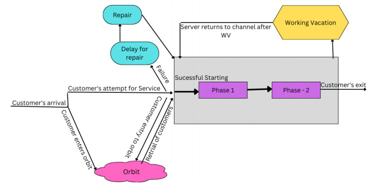
Related Papers:

[1]	M. Mossa Al-Sawalha, Saima Noor, Saleh Alshammari, Abdul Hamid Ganie, Ahmad Shafee . Analytical insights into solitary wave solutions of the fractional Estevez-Mansfield-Clarkson equation. AIMS Mathematics, 2024, 9(6): 13589-13606. doi: 10.3934/math.2024663
[2]	Naher Mohammed A. Alsafri . Solitonic behaviors in the coupled Drinfeld-Sokolov-Wilson system with fractional dynamics. AIMS Mathematics, 2025, 10(3): 4747-4774. doi: 10.3934/math.2025218
[3]	Mohammad Alqudah, Safyan Mukhtar, Albandari W. Alrowaily, Sherif. M. E. Ismaeel, S. A. El-Tantawy, Fazal Ghani . Breather patterns and other soliton dynamics in (2+1)-dimensional conformable Broer-Kaup-Kupershmit system. AIMS Mathematics, 2024, 9(6): 13712-13749. doi: 10.3934/math.2024669
[4]	Mahmoud Soliman, Hamdy M. Ahmed, Niveen Badra, Taher A. Nofal, Islam Samir . Highly dispersive gap solitons for conformable fractional model in optical fibers with dispersive reflectivity solutions using the modified extended direct algebraic method. AIMS Mathematics, 2024, 9(9): 25205-25222. doi: 10.3934/math.20241229
[5]	Chun Huang, Zhao Li . New soliton solutions of the conformal time derivative generalized $q$ -deformed sinh-Gordon equation. AIMS Mathematics, 2024, 9(2): 4194-4204. doi: 10.3934/math.2024206
[6]	Yanlin Li, Mohd Danish Siddiqi, Meraj Ali Khan, Ibrahim Al-Dayel, Maged Zakaria Youssef . Solitonic effect on relativistic string cloud spacetime attached with strange quark matter. AIMS Mathematics, 2024, 9(6): 14487-14503. doi: 10.3934/math.2024704
[7]	Gulnur Yel, Haci Mehmet Baskonus, Wei Gao . New dark-bright soliton in the shallow water wave model. AIMS Mathematics, 2020, 5(4): 4027-4044. doi: 10.3934/math.2020259
[8]	M. Mossa Al-Sawalha, Safyan Mukhtar, Azzh Saad Alshehry, Mohammad Alqudah, Musaad S. Aldhabani . Kink soliton phenomena of fractional conformable Kairat equations. AIMS Mathematics, 2025, 10(2): 2808-2828. doi: 10.3934/math.2025131
[9]	Yanlin Li, Dipen Ganguly, Santu Dey, Arindam Bhattacharyya . Conformal $\eta$ -Ricci solitons within the framework of indefinite Kenmotsu manifolds. AIMS Mathematics, 2022, 7(4): 5408-5430. doi: 10.3934/math.2022300
[10]	Chun Huang, Zhao Li . Soliton solutions of conformable time-fractional perturbed Radhakrishnan-Kundu-Lakshmanan equation. AIMS Mathematics, 2022, 7(8): 14460-14473. doi: 10.3934/math.2022797

Abstract

1. Introduction

Nonlinear fractional partial differential equations (NFPDEs) play a crucial role in the fields of applied science, engineering, and mathematics, as well as in modeling various physical nonlinear phenomena. The fields of fluid dynamics, fluid mechanics, neurons, optical fibers, electric circuits, water waves, plasma waves, capillary-gravity waves, chemical physics, and plasma physics have garnered significant attention due to the various fractional models developed ^[1,2]. Understanding the behaviors of distinct elements within various scientific fields is of the utmost significance, underscoring the necessity of exploring approaches to address non-functional partial differential equations (PDEs) ^[3,4,5].

The examination of soliton solutions to NFPDEs continues to hold academic significance, owing to the enhanced level of intricacy and comprehensiveness they provide compared to conventional solutions. A soliton can be defined as a solitary wave packet that exhibits self-reinforcing properties and traverses a medium without undergoing any changes in its shape or velocity. Fermion stability and robustness make them useful in many branches of physics and engineering. They facilitate the effective transmission of information and preserve coherence across long distances in nonlinear systems. Mathematicians have employed robust and various methodologies to pursue novel soliton solution outcomes. The notable methods include the Khater Ⅱ method ^[6], the modified Khater method ^[7], the ( $G^{\prime}/G$ )-expansion method ^[8], the $(G^{\prime2})$ -expansion method ^[9], the Kudryashov method ^[10,11], the Poincaré-Lighthill-Kuo method ^[12], the exp-function method ^[13], the fractional sub-equation method ^[14], the Sardar sub-equation method ^[15], the extended direct algebraic method (EDAM) ^{[16,17,18,19]}, and others.

In 1997, Mansfield and Clarkson introduced the Estevez-Mansfield-Clarkson Equation (EMCE), which is a nonlinear evolution equation of the fourth order ^[20]. This equation has proven advantageous in examining wave dynamics in shallow water, as it was initially employed in their investigation of pattern dispersion in liquid droplets. The EMCE is expressed in its formal form as follows:

$\begin{equation} \psi_{yyyt}+\varpi\psi_{yt}\psi_{y}+\varpi\psi_{yy}\psi_{t}+\psi _{tt} = 0. \end{equation}$

(1.1)

Here, $\psi\equiv\psi(y, t)$ indicates the wave function, and $\varpi$ is a non-zero constant. This study aims to create soliton solutions for the conformable EMCE (CEMCE) using the EDAM. This EMCE extension model substitutes integer-order derivatives with conformable fractional derivatives (CFDs). Numerous potential uses are introduced through the integration of CFDs in this framework. For example, CFDs, enable a more profound representation of the fractional-order kinetics present in some systems of matter that can enhance the precision of sims and forecasts. CFDs can help us better grasp the memory processes and non-local impacts prevalent in low-depth water interactions, which will help us simulate patterning generation, the dissemination of waves, and wave couplings in the EMCE. Implications for this improved system include tsunami modeling, coastal technology, research in the field of complicated hydrodynamics, and weather forecasting. Scholars can more effectively address real-world issues in related domains and get fresh knowledge into the behavior of shallow water swells by employing CFDs. The model is represented by the following equation ^[21]:

$\begin{equation} D_{t}^{\delta}(D_{y}^{\beta}(D_{y}^{\beta}(D_{y}^{\beta}\psi)))+\varpi D_{y}^{\beta}\psi D_{y}^{\beta}(D_{t}^{\delta}\psi)+\varpi D_{t}^{\delta}\psi D_{y}^{\beta}(D_{y}^{\beta}\psi)+D_{t}^{\delta}(D_{t}^{\delta}\psi ) = 0, \end{equation}$

(1.2)

where $D_{y}^{\beta}(\cdot)$ and $D_{t}^{\delta}(\cdot)$ are CFDs and $0 < \beta, \delta\leq1$ . CFDs provide an effective operator to explain the physical behavior of phenomena have a non-integer behavior, including occurrences that show effects of memory alongside their non-local and local behavior. In conventional math, localized behavior wherein the degree of shift at a location solely relies on its current surroundings is captured by conventional derivatives. Nonetheless, many systems in the real world exhibit non-local behavior, in which the system's past or remote locations impact the current condition of the structure at a given time. Fractional derivatives, including CFDs, extend calculus to explain such a behavior. For example, fractional interactions are a property of viscoelastic substances in the field of materials, wherein the tension or strain at a place depends on the material's distortion behavior and its current environment ^[22,23]. CFDs, which consider the entire system's behavior throughout an uninterrupted variety of past events, precisely represent this memory impact. Furthermore, the propagation of molecules in the diffusion process frequently exhibits non-local patterns. This results in fractional diffusing problems, where the spread of molecules across a non-local region determines the degree to which intensity changes occur at a given place. To accurately simulate these kinds of occurrences, CFDs offer a mathematical tool that bridges the gap between local and non-local behaviors and considers memory-related factors that are part of the system's behavior ^[24,25,26].

Prior to the present study, numerous scholars have dealt with the EMCE and the fractional EMCE (FEMCE). For example, the Kudryashov approach ^[21] yielded solutions to the nonlinear fractional space-time FEMCE, which formed exponential functions. Kinks and periodic waves characterized the behaviors found in the solution. The space-time fractional Ablowitz-Kaup-Newell-Segur (AKNS) water equation and the exact traveling wave solutions FEMCE were investigated by Phoosree & Chinviriyasit using the ( $G^{\prime}/G$ )-expansion approach in terms of hyperbolic functions, trigonometric functions, and rational functions ^[27]. Ultimately, Phoosree and Thadee ^[28] were able to obtain traveling wave solutions for the FEMCE by employing Jumarie's Riemann-Liouville derivative, thereby establishing the solution in the finite series, along with the simple equation technique and the Bernoulli equation. However in the present study, we will construct soliton solutions for the FEMCE using a novel EDAM approach. The recommended method transforms NFPDEs into nonlinear ordinary differential equations (NODEs) using Riccati Ordinary Differential Equations (ODE) and a finite series solution. This investigation has led to the discovery of soliton solutions that exhibit various mathematical structures, including trigonometric, exponential, rational, and hyperbolic functions. These structures allow for a detailed examination of their actual wave behaviors. In particular, we show that these behaviors are periodic, shock, and kink solitons. This is supported by showing how they look in contour, 3D, and 2D graphs. Interestingly, our results produce a wider variety of results than previous solutions, thus providing new and significant insights into the underlying phenomena of the model under study.

The rest of this investigation is organized in the following sections: Section 2 describes the materials and methodology for the EDAM; Section 3 shows the soliton solutions for the CEMCE; Section 4 includes a discussion and the corresponding graphics; and in Section 5, the most important findings are summarized in brief points.

2. Methodology & materials

2.1. The basic definition for the conformable fractional derivatives (CFDs)

By using the distinct advantages CFDs offer over other fractional derivative operators, it is possible to explicitly solve NFPDEs. Remarkably, different formulations of the fractional derivative for Eq (1.2) do not produce traveling wave and soliton solutions because they violate the chain rule ^[29,30]. Consequently, Eq (1.2) was modified to include the CFDs operator of order $\beta$ as follows ^[31]:

$\begin{equation} D_{\vartheta}^{\beta}w(\vartheta) = \lim\limits_{\gamma\rightarrow0}\frac {w(\gamma\vartheta^{1-\beta}+\vartheta)-w(\vartheta)}{\gamma}, \quad\beta \in(0, 1]. \end{equation}$

(2.1)

Here, we employ the following attributes of this derivative:

$\begin{equation} D_{\vartheta}^{\beta}\vartheta^{a} = a\vartheta^{a-\beta}, \end{equation}$

(2.2)

$\begin{equation} D_{\vartheta}^{\beta}(a_{1}\rho(\vartheta)\pm a_{2}\eta(\vartheta )) = a_{1}D_{\vartheta}^{\beta}(\rho(\vartheta))\pm a_{2}D_{\vartheta}^{\beta }(\eta(\vartheta)), \end{equation}$

(2.3)

$\begin{equation} D_{\vartheta}^{\beta}\chi\lbrack\zeta(\vartheta)] = \chi_{\zeta}^{\prime} (\zeta(\vartheta))D_{\vartheta}^{\beta}\zeta(\vartheta), \end{equation}$

(2.4)

where $\rho(\vartheta)$ , $\eta(\vartheta)$ , $\chi(\vartheta)$ , and $\zeta(\vartheta)$ are arbitrary differentiable functions, whereas $\left(a, a_{1}, a_{2}\right)$ are constants.

2.2. The working procedure of the EDAM

Here, we outline the operating strategy of the EDAM. Consider the following conditions and factors when working with the NFPDE:

$\begin{equation} R(\psi, D_{t}^{\alpha}\psi, D_{y_{1}}^{\beta}\psi, D_{y_{2}}^{\gamma}\psi, \psi D_{y_{1}}^{\beta}\psi, \ldots) = 0, \ \ 0 < \alpha, \beta, \gamma\leq1, \end{equation}$

(2.5)

where $\psi\equiv\psi(t, y_{1}, y_{2}, y_{3}, \ldots, y_{r})$ .

The following procedures are applied to solve Eq (2.5):

(1) We begin with a variable transformation of the type $\psi(t, y_{1}, y_{2}, y_{3}, \dots, y_{r})\equiv\Psi(\vartheta)$ , where $\vartheta$ can be written in several ways. This transformation converts the NFPDE (2.5) into the following NODE:

$\begin{equation} Q(\Psi, \Psi^{\prime}\Psi, \Psi^{\prime}, \dots) = 0, \end{equation}$

(2.6)

where $\Psi^{\prime} = \frac{d\Psi}{d\vartheta}$ .

Equation (2.6) may occasionally be integrated to make the NODE suitable for the homogenous balance principle.

(2) After that, by using the Riccati ODE, we consider the subsequent series-based solution to the NODE in Eq (2.6):

$\begin{equation} \Psi(\vartheta) = \sum\limits_{\sigma = -q}^{q}p_{\sigma}\zeta(\vartheta)^{\sigma}. \end{equation}$

(2.7)

In this context, $p_{\sigma}(\sigma = -q, ..., q)$ denotes the unknown constants, and $\zeta(\vartheta)$ is the general solution of the resulting ODE:

$\begin{equation} \zeta^{\prime}(\vartheta) = \lambda+\mu\zeta(\vartheta)+\nu\zeta(\vartheta)^{2}, \end{equation}$

(2.8)

where $\left(\lambda, \mu, \nu\right)$ are invariable.

(3) By creating a homogeneous balance for Eq (2.6) between the largest nonlinearity and the highest-order derivative, the positive integer $q$ introduced in Eq (2.7) is finally obtained.

(4) After that, we insert Eq (2.7) into either Eq (2.6) or the equation that arises from the integration of Eq (2.6) and combine the terms of $\zeta(\vartheta)$ into equivalent orders. This method results in an equation that includes $\zeta(\vartheta)$ . Then, the coefficients in this expression are set to zero, producing an algebraic system of equations for the variables $p_{\sigma}(\sigma = -q, ..., q)$ and other associated parameters.

(5) We apply MAPLE to solve this system of nonlinear algebraic equations.

(6) Then, the analytical soliton solutions for Eq (2.5) are then derived by computing and substituting the unknown values into Eq (2.7), together with the $\zeta(\vartheta)$ (the solution of Eq (2.8)). We can create the resulting families of soliton solutions using the general solution of Eq (2.8).

Family 1: For $M\left( = \mu^{2}-4\nu\lambda\right) < 0$ & $\nu\neq0$ , we obtain the following:

$\begin{align*} \zeta_{1}(\vartheta) & = -{\frac{\mu}{2\nu}}+{\frac{\sqrt{-M}}{2\nu}} \tan\left( \frac{1}{2}\, \sqrt{-M}\vartheta\right), \\ \zeta_{2}(\vartheta) & = -{\frac{\mu}{2\nu}}-{\frac{\sqrt{-M}}{2\nu}} \cot\left( \frac{1}{2}\, \sqrt{-M}\vartheta\right) , \\ \zeta_{3}(\vartheta) & = -{\frac{\mu}{2\nu}}+{\frac{\sqrt{-M}}{2\nu}}\left[ \tan\left( \sqrt{-M}\vartheta\right) +\sec\left( \sqrt{-M}\vartheta\right) \right] , \\ \zeta_{4}(\vartheta) & = -{\frac{\mu}{2\nu}}-{\frac{\sqrt{-M}}{2\nu}}\left[ \cot\left( \sqrt{-M}\vartheta\right) +\csc\left( \sqrt{-M}\vartheta\right) \right] , \\ \zeta_{5}(\vartheta) & = -{\frac{\mu}{2\nu}}+{\frac{\sqrt{-M}}{4\nu}}\left[ \tan\left( \frac{1}{4}\, \sqrt{-M}\vartheta\right) -\cot\left( \frac{1} {4}\, \sqrt{-M}\vartheta\right) \right] . \end{align*}$

Family 2: For $M > 0$ & $\nu\neq0$ , we obtain the following:

$\begin{align*} \zeta_{6}(\vartheta) & = -{\frac{\mu}{2\nu}}-{\frac{\sqrt{M}}{2\nu}} \tanh\left( \frac{1}{2}\, \sqrt{M}\vartheta\right) , \\ \zeta_{7}(\vartheta) & = -{\frac{\mu}{2\nu}}-{\frac{\sqrt{M}}{2\nu}} \coth\left( \frac{1}{2}\, \sqrt{M}\vartheta\right) , \\ \zeta_{8}(\vartheta) & = -{\frac{\mu}{2\nu}}-{\frac{\sqrt{M}}{2\nu}}\left[ \tanh\left( \sqrt{M}\vartheta\right) +\mathit{sech}\left( \sqrt{M} \vartheta\right) \right] , \\ \zeta_{9}(\vartheta) & = -{\frac{\mu}{2\nu}}-{\frac{\sqrt{M}}{2\nu}}\left[ \coth\left( \sqrt{M}\vartheta\right) +\mathit{csch}\left( \sqrt{M} \vartheta\right) \right] , \\ \zeta_{10}(\vartheta) & = -{\frac{\mu}{2\nu}}-{\frac{\sqrt{M}}{4\nu}}\left[ \tanh\left( \frac{1}{4}\, \sqrt{M}\vartheta\right) -\coth\left( \frac{1} {4}\, \sqrt{M}\vartheta\right) \right] . \end{align*}$

Family 3: For $\nu\lambda > 0$ & $\mu = 0$ , we obtain the following:

$\begin{align*} \zeta_{11}(\vartheta) & = \sqrt{{\frac{\lambda}{\nu}}}\tan\left( \sqrt{\lambda\nu}\vartheta\right) , \\ \zeta_{12}(\vartheta) & = -\sqrt{{\frac{\lambda}{\nu}}}\cot\left( \sqrt{\lambda\nu}\vartheta\right) , \\ \zeta_{13}(\vartheta) & = \sqrt{{\frac{\lambda}{\nu}}}\left[ \tan\left( 2\, \sqrt{\lambda\nu}\vartheta\right) +\sec\left( 2\, \sqrt{\lambda\nu }\vartheta\right) \right] , \\ \zeta_{14}(\vartheta) & = -\sqrt{{\frac{\lambda}{\nu}}}\left[ \cot\left( 2\, \sqrt{\lambda\nu}\vartheta\right) +\csc\left( 2\, \sqrt{\lambda\nu }\vartheta\right) \right] , \\ \zeta_{15}(\vartheta) & = \frac{1}{2}\sqrt{{\frac{\lambda}{\nu}}}\left[ \tan\left( \frac{1}{2}\, \sqrt{\lambda\nu}\vartheta\right) -\cot\left( \frac{1}{2}\, \sqrt{\lambda\nu}\vartheta\right) \right] . \end{align*}$

Family 4: For $\lambda\nu < 0$ and $\mu = 0$ , we obtain the following:

$\begin{align*} \zeta_{16}(\vartheta) & = -\sqrt{-{\frac{\lambda}{\nu}}}\tanh\left( \sqrt{-\lambda\nu}\vartheta\right) , \\ \zeta_{17}(\vartheta) & = -\sqrt{-{\frac{\lambda}{\nu}}}\coth\left( \sqrt{-\lambda\nu}\vartheta\right) , \\ \zeta_{18}(\vartheta) & = -\sqrt{-{\frac{\lambda}{\nu}}}\left[ \tanh\left( 2\, \sqrt{-\lambda\nu}\vartheta\right) +i\mathit{sech}\left( 2\, \sqrt {-\lambda\nu}\vartheta\right) \right] , \\ \zeta_{19}(\vartheta) & = -\sqrt{-{\frac{\lambda}{\nu}}}\left[ \coth\left( 2\, \sqrt{-\lambda\nu}\vartheta\right) +\mathit{csch}\left( 2\, \sqrt {-\lambda\nu}\vartheta\right) \right] , \\ \zeta_{20}(\vartheta) & = -\frac{1}{2}\sqrt{-{\frac{\lambda}{\nu}}}\left[ \tanh\left( \frac{1}{2}\, \sqrt{-\lambda\nu}\vartheta\right) +\coth\left( \frac{1}{2}\, \sqrt{-\lambda\nu}\vartheta\right) \right] . \end{align*}$

Family 5: For $\lambda = \nu$ & $\mu = 0$ , we obtain the following:

$\zeta_{21}(\vartheta) = \tan\left( \lambda\vartheta\right) ,$

$\zeta_{22}(\vartheta) = -\cot\left( \lambda\vartheta\right) ,$

$\zeta_{23}(\vartheta) = \tan\left( 2\, \lambda\vartheta\right) +\sec\left( 2\, \lambda\vartheta\right) ,$

$\zeta_{24}(\vartheta) = -\cot\left( 2\, \lambda\vartheta\right) +\csc\left( 2\, \lambda\vartheta\right) ,$

and

$\zeta_{25}(\vartheta) = \frac{1}{2}\tan\left( \frac{1}{2}\, \lambda \vartheta\right) -\frac{1}{2}\, \cot\left( \frac{1}{2}\, \lambda \vartheta\right) .$

Family 6: For $\nu = -\lambda$ & $\mu = 0$ , we obtain the following:

$\begin{align*} \zeta_{26}(\vartheta) & = -\tanh\left( \lambda\vartheta\right) , \\ \zeta_{27}(\vartheta) & = -\coth\left( \lambda\vartheta\right) , \\ \zeta_{28}(\vartheta) & = -\tanh\left( 2\, \lambda\vartheta\right) +i\mathit{sech}\left( 2\, \lambda\vartheta\right) , \\ \zeta_{29}(\vartheta) & = -\coth\left( 2\, \lambda\vartheta\right) +\mathit{csch}\left( 2\, \lambda\vartheta\right) , \\ \zeta_{30}(\vartheta) & = -\frac{1}{2}\tanh\left( \frac{1}{2}\, \lambda \vartheta\right) -\frac{1}{2}\, \coth\left( \frac{1}{2}\, \lambda \vartheta\right) . \end{align*}$

Family 7: For $M = 0$ , we obtain the following:

$\zeta_{31}(\vartheta) = -2\, {\frac{\lambda\left( \mu\vartheta\, +2\right) }{{\mu}^{2}\vartheta\, }}.$

Family 8: For $\mu = \tau$ , $\lambda = h\tau(h\neq0)$ & $\nu = 0$ , we obtain the following:

$\zeta_{32}(\vartheta) = {e}^{\tau\, \vartheta}-h.$

Family 9: For $\mu = \nu = 0$ , we obtain the following:

$\zeta_{33}(\vartheta) = \vartheta\, \lambda.$

Family 10: For $\mu = \lambda = 0$ , we obtain the following:

$\zeta_{34}(\vartheta) = -{\frac{1}{\vartheta\, \nu}}.$

Family 11: For $\lambda = 0$ , $\mu\neq0$ & $\nu\neq0$ , we obtain the following:

$\zeta_{35}(\vartheta) = -{\frac{\mu}{\nu\left( 1+\cosh\left( \mu \vartheta\right) -\sinh\left( \mu\vartheta\right) \right) }},$

and

$\zeta_{36}(\vartheta) = -{\frac{\mu\left[ \cosh\left( \mu\vartheta\right) +\sinh\left( \mu\vartheta\right) \right] }{\nu\left[ \cosh\left( \mu\vartheta\right) +\sinh\left( \mu\vartheta\right) +1\right] }}.$

Family 12: For $\mu = \tau$ , $\nu = h\tau(h\neq0)$ & $\lambda = 0$ , we obtain the following:

$\zeta_{37}(\vartheta) = {\frac{{e}^{\upsilon\, \vartheta}}{1-h{e}^{\upsilon \vartheta}}}.$

3. Execution of EDAM to CEMCE

In this study phase, the EDAM is employed to create soliton solutions for the CEMCE, as depicted in Eq (1.2). To initiate the technique, one must perform the following variable transformation:

$\begin{equation} \psi(x, y, t)\equiv\Psi(\vartheta)\;\text{with }\vartheta = \frac{\epsilon x^{\alpha}}{\alpha}+\frac{\kappa y^{\beta}}{\beta}-\frac{\omega t^{\delta} }{\delta}, \end{equation}$

(3.1)

which, with the help of Eqs (2.2) and (2.4), we have the following:

$\begin{split} & D_{t}^{\delta}\psi = D_{t}^{\delta}\Psi(\vartheta) = \Psi_{t}^{\prime\delta }(\vartheta) = -\omega\Psi^{\prime}(\vartheta), \\ & D_{t}^{\delta}(D_{t}^{\delta}\psi) = D_{t}^{\delta}(-\omega\Psi^{\prime }(\vartheta)) = -\omega\Psi_{t}^{\prime\prime\delta}\vartheta = \omega^{2} \Psi^{\prime\prime}(\vartheta), \\ & D_{y}^{\beta}\psi = D_{y}^{\beta}\Psi(\vartheta) = \Psi_{y}^{\prime\beta }(\vartheta) = \kappa\Psi^{\prime}(\vartheta), \\ & D_{y}^{\beta}(D_{y}^{\beta}\psi) = D_{y}^{\beta}(\kappa\Psi^{\prime }(\vartheta)) = \kappa\Psi_{y}^{\prime\prime\beta}\vartheta = \kappa^{2} \Psi^{\prime\prime}(\vartheta), \\ & D_{y}^{\beta}(D_{y}^{\beta}(D_{y}^{\beta}\psi)) = D_{y}^{\beta}(\kappa ^{2}\Psi^{\prime\prime2}\Psi_{y}^{\prime\prime\prime\beta}\vartheta = \kappa ^{3}\Psi^{\prime\prime\prime}(\vartheta), \\ & D_{y}^{\beta}(D_{y}^{\beta}(D_{y}^{\beta}(D_{y}^{\beta}\psi))) = D_{y} ^{\beta}(\kappa^{3}\Psi^{\prime\prime\prime3}\Psi^{(iv)}(\vartheta )D_{y}^{\beta}\vartheta = \kappa^{4}\Psi^{(iv)}(\vartheta), \\ & D_{t}^{\delta}(D_{y}^{\beta}\psi) = D_{t}^{\delta}(\kappa\Psi^{\prime }(\vartheta)) = \kappa\Psi_{t}^{\prime\prime\delta}\vartheta = -\omega\kappa \Psi^{\prime\prime}(\vartheta), \\ & D_{t}^{\delta}(D_{y}^{\beta}(D_{y}^{\beta}(D_{y}^{\beta}\psi))) = D_{t} ^{\delta}(\kappa^{3}\Psi^{\prime\prime\prime3}\Psi^{(iv)}(\vartheta )D_{t}^{\delta}\vartheta = -\omega\kappa^{3}\Psi^{(iv)}(\vartheta). \end{split}$

Now, by collecting all the above terms and adding them in Eq (1.2), the following NODE is obtained:

$\begin{equation} -\kappa^{3}\Psi^{(iv)}-2\kappa^{2}\varpi\Psi^{\prime}\Psi^{\prime\prime }+\omega\Psi^{\prime\prime} = 0. \end{equation}$

(3.2)

It is essential to observe that the variable transformation (3.1) is expressed in a two-dimensional format, although our problem is one-dimensional. Therefore, we can disregard the second dimension when performing our computations, (i.e., $\vartheta = \frac{\kappa y^{\beta}}{\beta }-\frac{\omega t^{\delta}}{\delta}$ ).

The result obtained from a single integration of Eq (3.2) with a constant of integration of zero is as follows:

$\begin{equation} -\kappa^{3}\Psi^{\prime\prime\prime}-\kappa^{2}\varpi\left( \Psi^{\prime }\right) ^{2}+\omega\Psi^{\prime} = 0. \end{equation}$

(3.3)

Upon constructing a homogeneous balancing condition between $\Psi ^{\prime\prime\prime}\longmapsto$ ( $3q$ ) and $(\left(\Psi^{\prime}\right) ^{2}$ $\longmapsto$ ( $q+2$ ), we conclude that $q$ $= 1$ . We obtain the following series-based solution for Eq (3.3) by substituting $q = 1$ into Eq (2.7):

$\begin{equation} \Psi(\vartheta) = \sum\limits_{\sigma = -1}^{1}p_{\sigma}\zeta(\vartheta)^{\sigma} = p_{-1}\zeta(\vartheta)^{-1}+p_{0}+p_{1}\zeta(\vartheta). \end{equation}$

(3.4)

We obtain an expression in $\zeta(\vartheta)$ by inserting Eq (3.4) into Eq (3.3) and accumulating the terms with similar powers of $\zeta (\vartheta)$ . The procedure produces a set of algebraic nonlinear equations when the coefficients are set to zero. When MAPLE is employed to solve this system, the two sets of solutions provided are as follows:

Case 1.

$\begin{equation} p_{{0}} = p_{{0}}, p_{{1}} = 0, p_{{-1}} = 3\, {\frac{\kappa\, \lambda}{\varpi}} , \omega = {\kappa}^{3}M, \kappa = \kappa. \end{equation}$

(3.5)

Case 2.

$\begin{equation} p_{{0}} = p_{{0}}, p_{{1}} = p_{{1}}, p_{{-1}} = 0, \omega = {\frac{-{\varpi}^{3}{p_{{1} }}^{3}M}{27{\nu}^{3}}}, \kappa = {\frac{-\varpi\, p_{{1}}}{3\nu}}. \end{equation}$

(3.6)

Now, we find all solutions for the two above cases.

Given case 1, we create the families of soliton solutions for the CEMCE (1.2) by employing Eqs (3.1) and (3.4) and the associated solution of Eq (2.8):

Family 1.1: For $M < 0\quad\nu\neq0$ , we obtain the following:

$\begin{equation} \psi_{1, 1} = \frac{3\, \kappa\, \lambda}{\varpi}\left[ -\frac{1}{2}\, {\frac{\mu }{\nu}}+\frac{1}{2}\, {\frac{\sqrt{-M}\tan\left( \frac{1}{2}\, \sqrt {-M}\vartheta\right) }{\nu}}\right] ^{-1}+p_{{0}}, \end{equation}$

(3.7)

$\begin{equation} \psi_{1, 2} = \frac{3\, \kappa\, \lambda}{\varpi}\left[ -\frac{1}{2}\, {\frac{\mu }{\nu}}-\frac{1}{2}\, {\frac{\sqrt{-M}\cot\left( \frac{1}{2}\, \sqrt {-M}\vartheta\right) }{\nu}}\right] ^{-1}+p_{{0}}, \end{equation}$

(3.8)

$\begin{equation} \psi_{1, 3} = \frac{3\, \kappa\, \lambda}{\varpi}\left[ -\frac{1}{2}\, {\frac{\mu }{\nu}}+\frac{1}{2}\, {\frac{\sqrt{-M}\left( \tan\left( \sqrt{-M} \vartheta\right) +\sec\left( \sqrt{-M}\vartheta\right) \right) }{\nu} }\right] ^{-1}+p_{{0}}, \end{equation}$

(3.9)

$\begin{equation} \psi_{1, 4} = \frac{3\, \kappa\, \lambda}{\varpi}\left[ -\frac{1}{2}\, {\frac{\mu }{\nu}}-\frac{1}{2}\, {\frac{\sqrt{-M}\left( \cot\left( \sqrt{-M} \vartheta\right) +\csc\left( \sqrt{-M}\vartheta\right) \right) }{\nu} }\right] ^{-1}+p_{{0}}, \end{equation}$

(3.10)

and

$\begin{equation} \psi_{1, 5} = \frac{3\, \kappa\, \lambda}{\varpi}\left[ -\frac{1}{2}\, {\frac{\mu }{\nu}}+\frac{1}{4}\, {\frac{\sqrt{-M}\left( \tan\left( \frac{1}{4} \, \sqrt{-M}\vartheta\right) -\cot\left( \frac{1}{4}\, \sqrt{-M} \vartheta\right) \right) }{\nu}}\right] ^{-1}+p_{{0}}. \end{equation}$

(3.11)

Family 1.2: For $M > 0\quad\nu\neq0$ , we obtain the following:

$\begin{equation} \psi_{1, 6} = \frac{3\, \kappa\, \lambda}{\varpi}\left[ -\frac{1}{2}\, {\frac{\mu }{\nu}}-\frac{1}{2}\, {\frac{\sqrt{M}\tanh\left( \frac{1}{2}\, \sqrt {M}\vartheta\right) }{\nu}}\right] ^{-1}+p_{{0}}, \end{equation}$

(3.12)

$\begin{equation} \psi_{1, 7} = \frac{3\, \kappa\, \lambda}{\varpi}\left[ -\frac{1}{2}\, {\frac{\mu }{\nu}}-\frac{1}{2}\, {\frac{\sqrt{M}\coth\left( \frac{1}{2}\, \sqrt {M}\vartheta\right) }{\nu}}\right] ^{-1}+p_{{0}}, \end{equation}$

(3.13)

$\begin{equation} \psi_{1, 8} = \frac{3\, \kappa\, \lambda}{\varpi}\left[ -\frac{1}{2}\, {\frac{\mu }{\nu}}-\frac{1}{2}\, {\frac{\sqrt{M}\left( \tanh\left( \sqrt{M} \vartheta\right) +i\mathit{sech}\left( \sqrt{M}\vartheta\right) \right) }{\nu}}\right] ^{-1}+p_{{0}}, \end{equation}$

(3.14)

$\begin{equation} \psi_{1, 9} = \frac{3\, \kappa\, \lambda}{\varpi}\left[ -\frac{1}{2}\, {\frac{\mu }{\nu}}-\frac{1}{2}\, {\frac{\sqrt{M}\left( \coth\left( \sqrt{M} \vartheta\right) +\mathit{csch}\left( \sqrt{M}\vartheta\right) \right) }{\nu}}\right] ^{-1}+p_{{0}}, \end{equation}$

(3.15)

and

$\begin{equation} \psi_{1, 10} = \frac{3\, \kappa\, \lambda}{\varpi}\left[ -\frac{1}{2}\, {\frac{\mu }{\nu}}-\frac{1}{4}\, {\frac{\sqrt{M}\left[ \tanh\left( \frac{1}{4}\, \sqrt {M}\vartheta\right) -\coth\left( \frac{1}{4}\, \sqrt{M}\vartheta\right) \right] }{\nu}}\right] ^{-1}+p_{{0}}. \end{equation}$

(3.16)

Family 1.3: For $\lambda\nu > 0$ and $\mu = 0$ , we obtain the following:

$\begin{equation} \psi_{1, 11} = \frac{3\, \kappa\, }{\varpi}\sqrt{\lambda\nu}\left( \tan\left( \sqrt{\lambda\, \nu}\vartheta\right) \right) ^{-1}+p_{{0}}, \end{equation}$

(3.17)

$\begin{equation} \psi_{1, 12} = -\frac{3\, \kappa\, }{\varpi}\sqrt{\lambda\nu}\left( \cot\left( \sqrt{\lambda\, \nu}\vartheta\right) \right) ^{-1}+p_{{0}}, \end{equation}$

(3.18)

$\begin{equation} \psi_{1, 13} = \frac{3\, \kappa\, }{\varpi}\sqrt{\lambda\nu}\left( \tan\left( 2\, \sqrt{\lambda\, \nu}\vartheta\right) +\sec\left( 2\, \sqrt{\lambda\, \nu }\vartheta\right) \right) ^{-1}+p_{{0}}, \end{equation}$

(3.19)

$\begin{equation} \psi_{1, 14} = -\frac{3\, \kappa\, }{\varpi}\sqrt{\lambda\nu}\left( \cot\left( 2\, \sqrt{\lambda\, \nu}\vartheta\right) +\csc\left( 2\, \sqrt{\lambda\, \nu }\vartheta\right) \right) ^{-1}+p_{{0}}, \end{equation}$

(3.20)

and

$\begin{equation} \psi_{1, 15} = \frac{6\, \kappa\, }{\varpi}\sqrt{\lambda\nu}\left( \tan\left( \frac{1}{2}\, \sqrt{\lambda\, \nu}\vartheta\right) -\cot\left( \frac{1} {2}\, \sqrt{\lambda\, \nu}\vartheta\right) \right) ^{-1}+p_{{0}}. \end{equation}$

(3.21)

Family 1.4: For $\lambda\nu < 0$ and $\mu = 0$ , we obtain the following:

$\begin{equation} \psi_{1, 16} = -\frac{3\, \kappa\, }{\varpi}\sqrt{-\lambda\nu}\left( \tanh\left( \sqrt{-\lambda\, \nu}\vartheta\right) \right) ^{-1}+p_{{0}}, \end{equation}$

(3.22)

$\begin{equation} \psi_{1, 17} = -\frac{3\, \kappa\, }{\varpi}\sqrt{-\lambda\nu}\left( \coth\left( \sqrt{-\lambda\, \nu}\vartheta\right) \right) ^{-1}+p_{{0}}, \end{equation}$

(3.23)

$\begin{equation} \psi_{1, 18} = -\frac{3\, \kappa\, }{\varpi}\sqrt{-\lambda\nu}\left( \tanh\left( 2\, \sqrt{-\lambda\, \nu}\vartheta\right) +i\mathit{sech}\left( 2\, \sqrt {-\lambda\, \nu}\vartheta\right) \right) ^{-1}+p_{{0}}, \end{equation}$

(3.24)

$\begin{equation} \psi_{1, 19} = -\frac{3\, \kappa\, }{\varpi}\sqrt{-\lambda\nu}\left( \coth\left( 2\, \sqrt{-\lambda\, \nu}\vartheta\right) +\mathit{csch}\left( 2\, \sqrt {-\lambda\, \nu}\vartheta\right) \right) ^{-1}+p_{{0}}, \end{equation}$

(3.25)

and

$\begin{equation} \psi_{1, 20} = \frac{-6\, \kappa\, }{\varpi}\sqrt{-\lambda\nu}\left( \tanh\left( \frac{1}{2}\, \sqrt{-\lambda\, \nu}\vartheta\right) +\coth\left( \frac{1} {2}\, \sqrt{-\lambda\, \nu}\vartheta\right) \right) ^{-1}+p_{{0}}. \end{equation}$

(3.26)

Family 1.5: For $\nu = \lambda$ and $\mu = 0$ , we obtain the following:

$\begin{equation} \psi_{1, 21} = 3\, {\frac{\kappa\, \lambda}{\varpi\, \tan\left( \lambda \, \vartheta\right) }}+p_{{0}}, \end{equation}$

(3.27)

$\begin{equation} \psi_{1, 22} = -3\, {\frac{\kappa\, \lambda}{\varpi\, \cot\left( \lambda \, \vartheta\right) }}+p_{{0}}, \end{equation}$

(3.28)

$\begin{equation} \psi_{1, 23} = 3\, {\frac{\kappa\, \lambda}{\varpi\, \left( \tan\left( 2\, \lambda\, \vartheta\right) +\sec\left( 2\, \lambda\, \vartheta\right) \right) }}+p_{{0}}, \end{equation}$

(3.29)

$\begin{equation} \psi_{1, 24} = 3\, {\frac{\kappa\, \lambda}{\varpi\, \left( -\cot\left( 2\, \lambda\, \vartheta\right) -\csc\left( 2\, \lambda\, \vartheta\right) \right) }}+p_{{0}}, \end{equation}$

(3.30)

and

$\begin{equation} \psi_{1, 25} = 3\, {\frac{\kappa\, \lambda}{\varpi\, \left( \frac{1}{2} \, \tan\left( \frac{1}{2}\, \lambda\, \vartheta\right) -\frac{1}{2} \, \cot\left( \frac{1}{2}\, \lambda\, \vartheta\right) \right) }}+p_{{0}}. \end{equation}$

(3.31)

Family 1.6: For $\nu = -\lambda$ and $\mu = 0$ , we obtain the following:

$\begin{equation} \psi_{1, 26} = -3\, {\frac{\kappa\, \lambda}{\varpi\, \tanh\left( \lambda \, \vartheta\right) }}+p_{{0}}, \end{equation}$

(3.32)

$\begin{equation} \psi_{1, 27} = -3\, {\frac{\kappa\, \lambda}{\varpi\, \coth\left( \lambda \, \vartheta\right) }}+p_{{0}}, \end{equation}$

(3.33)

$\begin{equation} \psi_{1, 28} = 3\, {\frac{\kappa\, \lambda}{\varpi\, \left( -\tanh\left( 2\, \lambda\, \vartheta\right) -i\mathit{sech}\left( 2\, \lambda\, \vartheta \right) \right) }}+p_{{0}}, \end{equation}$

(3.34)

$\begin{equation} \psi_{1, 29} = 3\, {\frac{\kappa\, \lambda}{\varpi\, \left( -\coth\left( 2\, \lambda\, \vartheta\right) -\mathit{csch}\left( 2\, \lambda\, \vartheta \right) \right) }}+p_{{0}}, \end{equation}$

(3.35)

and

$\begin{equation} \psi_{1, 30} = 3\, {\frac{\kappa\, \lambda}{\varpi\, \left( -\frac{1}{2} \, \tanh\left( \frac{1}{2}\, \lambda\, \vartheta\right) -\frac{1}{2} \, \coth\left( \frac{1}{2}\, \lambda\, \vartheta\right) \right) }}+p_{{0}}. \end{equation}$

(3.36)

Family 1.7: For $M = 0$ , we get

$\begin{equation} \psi_{1, 31} = -3/2\, {\frac{\kappa\, \lambda\, {\mu}^{2}\vartheta}{\varpi \, \lambda\left( \mu\, \vartheta+2\right) }}+p_{{0}}. \end{equation}$

(3.37)

Family 1.8: For $\mu = \tau$ , $\lambda = h\tau(h\neq0)$ and $\nu = 0$ ,

$\begin{equation} \psi_{1, 32} = {\frac{3\, \kappa\, h\tau+p_{{0}}\varpi\, {\mathrm{e}^{\tau \, \vartheta}}-p_{{0}}\varpi\, h}{\varpi\, \left( {\mathrm{e}^{\tau\, \vartheta} }-h\right) }}. \end{equation}$

(3.38)

Family 1.9: For $\mu = \nu = 0$ , we obtain the following:

$\begin{equation} \psi_{1, 33} = 3\, {\frac{\kappa}{\varpi\, \vartheta}}+p_{{0}}. \end{equation}$

(3.39)

According to case 1, the value of $\vartheta$ reads

$\vartheta = \frac{\kappa y^{\beta}}{\beta}-\frac{({\kappa}^{3}M)t^{\delta} }{\delta}.$

For case 2, and utilizing Eqs (3.1) and (3.4) with the corresponding solution of Eq (2.8), we construct the following families of traveling wave solutions for Eq (1.2):

Family 2.1: For $M < 0\quad\nu\neq0$ , we obtain the following:

$\begin{equation} \psi_{2, 1} = p_{{0}}+p_{{1}}\left( -\frac{1}{2}\, {\frac{\mu}{\nu}}+\frac{1} {2}\, {\frac{\sqrt{-M}\tan\left( \frac{1}{2}\, \sqrt{-M}\vartheta\right) } {\nu}}\right) , \end{equation}$

(3.40)

$\begin{equation} \psi_{2, 2} = p_{{0}}+p_{{1}}\left( -\frac{1}{2}\, {\frac{\mu}{\nu}}-\frac{1} {2}\, {\frac{\sqrt{-M}\cot\left( \frac{1}{2}\, \sqrt{-M}\vartheta\right) } {\nu}}\right) , \end{equation}$

(3.41)

$\begin{equation} \psi_{2, 3} = p_{{0}}+p_{{1}}\left( -\frac{1}{2}\, {\frac{\mu}{\nu}}+\frac{1} {2}\, {\frac{\sqrt{-M}\left( \tan\left( \sqrt{-M}\vartheta\right) +\sec\left( \sqrt{-M}\vartheta\right) \right) }{\nu}}\right) , \end{equation}$

(3.42)

$\begin{equation} \psi_{2, 4} = p_{{0}}+p_{{1}}\left( -\frac{1}{2}\, {\frac{\mu}{\nu}}-\frac{1} {2}\, {\frac{\sqrt{-M}\left( \cot\left( \sqrt{-M}\vartheta\right) +\csc\left( \sqrt{-M}\vartheta\right) \right) }{\nu}}\right) , \end{equation}$

(3.43)

and

$\begin{equation} \psi_{2, 5} = p_{{0}}+p_{{1}}\left( -\frac{1}{2}\, {\frac{\mu}{\nu}}+\frac{1} {4}\, {\frac{\sqrt{-M}\left( \tan\left( \frac{1}{4}\, \sqrt{-M}\vartheta \right) -\cot\left( 1/4\, \sqrt{-M}\vartheta\right) \right) }{\nu}}\right) . \end{equation}$

(3.44)

Family 2.2: For $M > 0\quad\nu\neq0$ , we obtain the following:

$\begin{equation} \psi_{2, 6} = p_{{0}}+p_{{1}}\left( -\frac{1}{2}\, {\frac{\mu}{\nu}}-\frac{1} {2}\, {\frac{\sqrt{M}\tanh\left( \frac{1}{2}\, \sqrt{M}\vartheta\right) }{\nu }}\right) , \end{equation}$

(3.45)

$\begin{equation} \psi_{2, 7} = p_{{0}}+p_{{1}}\left( -\frac{1}{2}\, {\frac{\mu}{\nu}}-\frac{1} {2}\, {\frac{\sqrt{M}\coth\left( \frac{1}{2}\, \sqrt{M}\vartheta\right) }{\nu }}\right) , \end{equation}$

(3.46)

$\begin{equation} \psi_{2, 8} = p_{{0}}+p_{{1}}\left( -\frac{1}{2}\, {\frac{\mu}{\nu}}-\frac{1} {2}\, {\frac{\sqrt{M}\left( \tanh\left( \sqrt{M}\vartheta\right) +i\mathit{sech}\left( \sqrt{M}\vartheta\right) \right) }{\nu}}\right) , \end{equation}$

(3.47)

$\begin{equation} \psi_{2, 9} = p_{{0}}+p_{{1}}\left( -\frac{1}{2}\, {\frac{\mu}{\nu}}-\frac{1} {2}\, {\frac{\sqrt{M}\left( \coth\left( \sqrt{M}\vartheta\right) +\mathit{csch}\left( \sqrt{M}\vartheta\right) \right) }{\nu}}\right) , \end{equation}$

(3.48)

and

$\begin{equation} \psi_{2, 10} = p_{{0}}+p_{{1}}\left( -\frac{1}{2}\, {\frac{\mu}{\nu}}-\frac{1} {4}\, {\frac{\sqrt{M}\left( \tanh\left( \frac{1}{4}\, \sqrt{M}\vartheta \right) -\coth\left( 1/4\, \sqrt{M}\vartheta\right) \right) }{\nu}}\right) . \end{equation}$

(3.49)

Family 2.3: For $\lambda\nu > 0$ and $\mu = 0$ , we obtain the following:

$\begin{equation} \psi_{2, 11} = p_{{0}}+p_{{1}}\sqrt{{\frac{\lambda}{\nu}}}\tan\left( \sqrt{\lambda\, \nu}\vartheta\right) , \end{equation}$

(3.50)

$\begin{equation} \psi_{2, 12} = p_{{0}}-p_{{1}}\sqrt{{\frac{\lambda}{\nu}}}\cot\left( \sqrt{\lambda\, \nu}\vartheta\right) , \end{equation}$

(3.51)

$\begin{equation} \psi_{2, 13} = p_{{0}}+p_{{1}}\sqrt{{\frac{\lambda}{\nu}}}\left( \tan\left( 2\, \sqrt{\lambda\, \nu}\vartheta\right) +\sec\left( 2\, \sqrt{\lambda\, \nu }\vartheta\right) \right) , \end{equation}$

(3.52)

$\begin{equation} \psi_{2, 14} = p_{{0}}-p_{{1}}\sqrt{{\frac{\lambda}{\nu}}}\left( \cot\left( 2\, \sqrt{\lambda\, \nu}\vartheta\right) +\csc\left( 2\, \sqrt{\lambda\, \nu }\vartheta\right) \right) , \end{equation}$

(3.53)

and

$\begin{equation} \psi_{2, 15} = p_{{0}}+\frac{1}{2}\, p_{{1}}\sqrt{{\frac{\lambda}{\nu}}}\left( \tan\left( \frac{1}{2}\, \sqrt{\lambda\, \nu}\vartheta\right) -\cot\left( \frac{1}{2}\, \sqrt{\lambda\, \nu}\vartheta\right) \right) . \end{equation}$

(3.54)

Family 2.4: For $\lambda\nu < 0$ and $\mu = 0$ , we obtain the following:

$\begin{equation} \psi_{2, 16} = p_{{0}}-p_{{1}}\sqrt{-{\frac{\lambda}{\nu}}}\tanh\left( \sqrt{-\lambda\, \nu}\vartheta\right) , \end{equation}$

(3.55)

$\begin{equation} \psi_{2, 17} = p_{{0}}-p_{{1}}\sqrt{-{\frac{\lambda}{\nu}}}\coth\left( \sqrt{-\lambda\, \nu}\vartheta\right) , \end{equation}$

(3.56)

$\begin{equation} \psi_{2, 18} = p_{{0}}-p_{{1}}\sqrt{-{\frac{\lambda}{\nu}}}\left( \tanh\left( 2\, \sqrt{-\lambda\, \nu}\vartheta\right) +i\mathit{sech}\left( 2\, \sqrt {-\lambda\, \nu}\vartheta\right) \right) , \end{equation}$

(3.57)

$\begin{equation} \psi_{2, 19} = p_{{0}}-p_{{1}}\sqrt{-{\frac{\lambda}{\nu}}}\left( \coth\left( 2\, \sqrt{-\lambda\, \nu}\vartheta\right) +\mathit{csch}\left( 2\, \sqrt {-\lambda\, \nu}\vartheta\right) \right) , \end{equation}$

(3.58)

and

$\begin{equation} \psi_{2, 20} = p_{{0}}-\frac{1}{2}\, p_{{1}}\sqrt{-{\frac{\lambda}{\nu}}}\left( \tanh\left( \frac{1}{2}\, \sqrt{-\lambda\, \nu}\vartheta\right) +\coth\left( \frac{1}{2}\, \sqrt{-\lambda\, \nu}\vartheta\right) \right) . \end{equation}$

(3.59)

Family 2.5: For $\nu = \lambda$ and $\mu = 0$ , we obtain the following:

$\begin{equation} \psi_{2, 21} = p_{{0}}+p_{{1}}\tan\left( \lambda\, \vartheta\right) , \end{equation}$

(3.60)

$\begin{equation} \psi_{2, 22} = p_{{0}}-p_{{1}}\cot\left( \lambda\, \vartheta\right) , \end{equation}$

(3.61)

$\begin{equation} \psi_{2, 23} = p_{{0}}+p_{{1}}\left( \tan\left( 2\, \lambda\, \vartheta\right) +\sec\left( 2\, \lambda\, \vartheta\right) \right) , \end{equation}$

(3.62)

$\begin{equation} \psi_{2, 24} = p_{{0}}+p_{{1}}\left( -\cot\left( 2\, \lambda\, \vartheta\right) -\csc\left( 2\, \lambda\, \vartheta\right) \right) , \end{equation}$

(3.63)

and

$\begin{equation} \psi_{2, 25} = p_{{0}}+p_{{1}}\left( \frac{1}{2}\, \tan\left( \frac{1} {2}\, \lambda\, \vartheta\right) -\frac{1}{2}\, \cot\left( \frac{1}{2} \, \lambda\, \vartheta\right) \right) . \end{equation}$

(3.64)

Family 2.6: For $\nu = -\lambda$ and $\mu = 0$ , we obtain the following:

$\begin{equation} \psi_{2, 26} = p_{{0}}-p_{{1}}\tanh\left( \lambda\, \vartheta\right) , \end{equation}$

(3.65)

$\begin{equation} \psi_{2, 27} = p_{{0}}-p_{{1}}\coth\left( \lambda\, \vartheta\right) , \end{equation}$

(3.66)

$\begin{equation} \psi_{2, 28} = p_{{0}}+p_{{1}}\left( -\tanh\left( 2\, \lambda\, \vartheta\right) -i\mathit{sech}\left( 2\, \lambda\, \vartheta\right) \right) , \end{equation}$

(3.67)

$\begin{equation} \psi_{2, 29} = p_{{0}}+p_{{1}}\left( -\coth\left( 2\, \lambda\, \vartheta\right) -\mathit{csch}\left( 2\, \lambda\, \vartheta\right) \right) , \end{equation}$

(3.68)

and

$\begin{equation} \psi_{2, 30} = p_{{0}}+p_{{1}}\left( -\frac{1}{2}\, \tanh\left( \frac{1} {2}\, \lambda\, \vartheta\right) -\frac{1}{2}\, \coth\left( \frac{1} {2}\, \lambda\, \vartheta\right) \right) . \end{equation}$

(3.69)

Family 2.7: For $M = 0$ , we obtain the following:

$\begin{equation} \psi_{2, 31} = p_{{0}}-2\, {\frac{p_{{1}}\lambda\left( \mu\, \vartheta+2\right) }{{\mu}^{2}\vartheta}}. \end{equation}$

(3.70)

Family 2.8: For $\lambda = \mu = 0$ , we obtain the following:

$\begin{equation} \psi_{2, 32} = p_{{0}}-{\frac{p_{{1}}}{\nu\, \vartheta}}. \end{equation}$

(3.71)

Family 2.9: For $\lambda = 0$ , $\mu\neq0$ and $\nu\neq0$ , we obtain the following:

$\begin{equation} \psi_{2, 33} = p_{{0}}-{\frac{p_{{1}}\mu}{\nu\, \left( \cosh\left( \mu\, \vartheta\right) -\sinh\left( \mu\, \vartheta\right) +1\right) }}, \end{equation}$

(3.72)

and

$\begin{equation} \psi_{2, 34} = p_{{0}}-{\frac{p_{{1}}\mu\, \left( \cosh\left( \mu\, \vartheta \right) +\sinh\left( \mu\, \vartheta\right) \right) }{\nu\, \left( \cosh\left( \mu\, \vartheta\right) +\sinh\left( \mu\, \vartheta\right) +1\right) }}. \end{equation}$

(3.73)

Family 2.10: For $\mu = \tau$ , $\nu = h\tau(h\neq0)$ and $\lambda = 0$ , we obtain the following:

$\begin{equation} \psi_{2, 35} = p_{{0}}+{\frac{p_{{1}}\mathrm{e^{\tau\, \vartheta}}} {1-h\mathrm{e^{\tau\, \vartheta}}}}. \end{equation}$

(3.74)

According to case 2, the value of $\vartheta$ reads obtain the following:

$\vartheta = \frac{({\frac{-\varpi\, p_{{1}}}{3\nu}})y^{\beta}}{\beta} -\frac{({\frac{-{\varpi}^{3}{p_{{1}}}^{3}M}{27{\nu}^{3}}})t^{\delta}}{\delta}.$

4. Discussion and graphs

This section provides graphic representations of various wave patterns for the model under consideration. The obtained solutions for different wave structures have been numerically examined in 3D and 2D forms using suitable values of the related parameters. We show that the obtained soliton solutions appear as periodic and kink wave solitons. Carefully choosing the parameters results in unique and educational visuals. Furthermore, the study's results are novel because, to the best of our knowledge, there is no prior literature that utilized this technique's results and applied them to the CEMCE. Moreover, it is essential to note that our analytical findings can be related to those derived from other approaches, such as the Riccati ODE expanding techniques, the F-expansion method, the tanh-method, and other related approaches, within specific limitations. Our work might be interpreted as a generalization of existing techniques, providing a more comprehensive framework from which these particular techniques can be drawn or comprehended.

The results obtained from the numerical investigations indicate that the soliton solutions developed can be classified into two main categories: Kink waves are distinguished by a restricted disruption or deflection in the wave pattern, which frequently retains its form throughout propagation; a periodic soliton is an autonomous wave propagating through a medium while preserving its shape and magnitude at regular intervals. Periodic, kink, and shock waves can display characteristics similar to wave breaking in shallow water waves. Wave breaking is a phenomenon that typically occurs near shorelines or other water barriers, and results in the sudden conversion of a wave into turbulent water. As a result, the generated soliton solutions provide valuable insights into the complex dynamics of the CEMCE and illustrate the fundamental principles that govern the interaction and propagation of the wave. By examining these solutions, academic researchers can enhance their comprehension of the model's performance in many contexts. These provide insights into phenomena such as the dispersion of configurations in liquid droplets and the behavior of waves in shallow water.

In this instance, we have conducted a graphical analysis of several derived aforementioned solutions to gain insights into the wave propagation mechanics and to enhance the reader's comprehension of the concept. For case (1), we numerically analyzed some of its solutions, as illustrated in –. In these figures, we studied and examined the effect of the fractional parameters $(\beta, \delta)$ on the wave profile described by these solutions. For instance, solution (3.12) was numerically analyzed, as shown in . The periodic wave solution (3.16) was analyzed, and the influence of the time-fractional parameter $\delta$ on the wave's behavior was investigated, as depicted in . Additionally, the impact of $\delta$ on the profile of the shock wave was investigated. Moreover, an investigation was conducted to examine the impact of $\delta$ on the characteristics of shock waves and solitons as specified by the solution (3.24). It is essential to acknowledge that the solution (3.24) exhibits complexity since it is comprised of both real and imaginary components. illustrates the shock wave, represented by the real part, and illustrates the solitons, represented by the imaginary part. Moreover, the absolute value of the solution (3.24) against $\delta$ was investigated, as shown in . The results obtained from the numerical analysis demonstrate that the time-fractional parameter exerts a substantial influence on the characteristics of both the shock waves and the soliton profiles. Additionally, another solution (3.26) for case (1) was examined, as depicted in . In this figure, we also studied the effect of $\delta$ on the profile of the shock waves described by solution (3.26).

Figure 1. The shock wave solution (3.12)

$\psi_{1, 6}$ is numerically investigated: (a) 3D graph in

$\left(y, t\right) -$ plane for

$\left(\beta, \delta\right) = \left(1, 0.7\right)$ , (b) 3D graph in

$\left(y, t\right) -$ plane for

$\left(\beta, \delta\right) = \left(1, 0.85\right)$ , (c) 3D graph in

$\left(y, t\right) -$ plane for

$\left(\beta, \delta\right) = \left(1, 1\right)$ , and (d) the solution (3.12) is plotted against

$y$ for different values of time-fractional parameter

$\delta$ and for

$\left(t, \beta\right) = \left(0.1, 1\right)$ . Here,

$\lambda = 0.01,$

$\mu = 4,$

$\nu = 0.1,$

$\varpi = 1,$

$p_{{0}} = 10$ , and

$k = 1$ .

DownLoad: Full-Size Img PowerPoint

Figure 2. The periodic solution (3.16)

$\psi_{1, 10}$ is numerically examined: (a) 3D graph in

$\left(y, t\right) -$ plane for

$\left(\beta, \delta\right) = \left(1, 0.2\right)$ , (b) 3D graph in

$\left(y, t\right) -$ plane for

$\left(\beta, \delta\right) = \left(1, 0.4\right)$ , (c) 3D graph in

$\left(y, t\right) -$ plane for

$\left(\beta, \delta\right) = \left(1, 1\right)$ , and (d) the solution (3.16) is plotted against

$y$ for different values of time-fractional parameter

$\delta$ and for

$\left(t, \beta\right) = \left(0.1, 1\right)$ . Here,

$\lambda = \nu = 0.1,$

$\mu = 0,$

$\varpi = 1,$

$p_{{0}} = 10$ , and

$k = 10$ .

DownLoad: Full-Size Img PowerPoint

Figure 3. The real part of solution (3.24) Re

$\left[\psi_{1, 18}\right]$ is numerically examined: (a) 3D graph for shock waves in

$\left(y, t\right) -$ plane for

$\left(\beta, \delta\right) = \left(1, 0.2\right)$ , (b) 3D graph for shock waves in

$\left(y, t\right) -$ plane for

$\left(\beta, \delta\right) = \left(1, 0.4\right)$ , (c) 3D graph for shock waves in

$\left(y, t\right) -$ plane for

$\left(\beta, \delta\right) = \left(1, 1\right)$ , and (d) the real part of shock wave solution (3.24) is plotted against

$y$ for different values of time-fractional parameter

$\delta$ and for

$\left(t, \beta\right) = \left(0.1, 1\right)$ . Here,

$\lambda = -2, \nu = 1,$

$\mu = 0,$

$\varpi = 3,$

$p_{{0}} = 0.1$ , and

$k = 0.25$ .

DownLoad: Full-Size Img PowerPoint

Figure 4. The imaginary part of solution (3.24) Im

$\left[\psi_{1, 18}\right]$ is numerically examined: (a) 3D graph for shock waves in

$\left(y, t\right) -$ plane for

$\left(\beta, \delta\right) = \left(1, 0.2\right)$ , (b) 3D graph for shock waves in

$\left(y, t\right) -$ plane for

$\left(\beta, \delta\right) = \left(1, 0.4\right)$ , (c) 3D graph for shock waves in

$\left(y, t\right) -$ plane for

$\left(\beta, \delta\right) = \left(1, 1\right)$ , and (d) the imaginary part of shock wave solution (3.24) is plotted against

$y$ for different values of time-fractional parameter

$\delta$ and for

$\left(t, \beta\right) = \left(0.1, 1\right)$ . Here,

$\lambda = -2, \nu = 1,$

$\mu = 0,$

$\varpi = 3,$

$p_{{0}} = 0.1$ , and

$k = 0.25$ .

DownLoad: Full-Size Img PowerPoint

Figure 5. The absolute value of solution (3.24)

$\left\vert \psi_{1, 18}\right\vert$ is numerically examined: (a) 3D graph for shock waves in

$\left(y, t\right) -$ plane for

$\left(\beta, \delta\right) = \left(1, 0.2\right)$ , (b) 3D graph for shock waves in

$\left(y, t\right) -$ plane for

$\left(\beta, \delta\right) = \left(1, 0.4\right)$ , (c) 3D graph for shock waves in

$\left(y, t\right) -$ plane for

$\left(\beta, \delta\right) = \left(1, 1\right)$ , and (d) the absolute value of shock wave solution (3.24) is plotted against

$y$ for different values of time-fractional parameter

$\delta$ and for

$\left(t, \beta\right) = \left(0.1, 1\right)$ . Here,

$\lambda = -2, \nu = 1,$

$\mu = 0,$

$\varpi = 3,$

$p_{{0}} = 0.1$ , and

$k = 0.25$ .

DownLoad: Full-Size Img PowerPoint

Figure 6. Solution (3.26)

$\psi_{1, 20}$ is numerically investigated: (a) 3D graph in

$\left(y, t\right) -$ plane for

$\left(\beta, \delta\right) = \left(1, 0.1\right)$ , (b) 3D graph in

$\left(y, t\right) -$ plane for

$\left(\beta, \delta\right) = \left(1, 0.2\right)$ , (c) 3D graph in

$\left(y, t\right) -$ plane for

$\left(\beta, \delta\right) = \left(1, 1\right)$ , and (d) the solution (3.26) is plotted against

$y$ for different values of time-fractional parameter

$\delta$ and for

$\left(t, \beta\right) = \left(0.1, 1\right)$ . Here,

$\lambda = -2,$

$\mu = 0,$

$\nu = 1,$

$\varpi = 3,$

$p_{{0} } = 0.10$ , and

$k = 0.25$ .

DownLoad: Full-Size Img PowerPoint

To investigate the impact of the space-fractional parameter $\beta$ on the behavior of various solutions, we analyzed solutions (3.12), (3.16), (3.24), and (3.26), as depicted in . This diagram illustrates the susceptibility of these solutions to $\beta$ , which significantly influences the alteration of the waves behavior represented by these solutions. Furthermore, in this investigation, an examination was conducted on several solutions of case (2), as depicted in Figures 8–. For instance, we analyzed solution (3.45) and examined the impact of the time-fractional parameter on the properties of the shock waves described by this solution, as depicted in . Additionally, we analyzed the complex solution (3.47) and studied the effect of $\delta$ on the profile of the real and imaginary parts of this solution, as well as its absolute value, as illustrated in Figures 9–11, respectively. Moreover, we analyzed solutions (3.55), (3.65), (3.72), and (3.73) and examined the impact of the time-fractional parameter on the characteristics of shock waves, as depicted in Figures 12–15, respectively.

Figure 7. The impact of space-fractional parameter

$\beta$ on the profile of solutions (3.12), (3.16), (3.24), and (3.26) is numerically investigated: (a) solution (3.12) for

$\lambda = 0.01,$

$\mu = 4,$

$\nu = 0.1,$

$\varpi = 1,$

$p_{{0}} = 10$ ,

$k = 1$ ,

$y = 0.1$ , and

$\delta = 1$ , (b) solution (3.16) for

$\lambda = \nu = 0.1,$

$\mu = 0,$

$\varpi = 1,$

$p_{{0}} = 10$ ,

$k = 10$ ,

$y = 0.1$ , and

$\delta = 1$ , (c) solution (3.24) for

$\lambda = -2, \nu = 1,$

$\mu = 0,$

$\varpi = 3,$

$p_{{0}} = 0.1$ ,

$k = 0.25$ ,

$y = 0.1$ , and

$\delta = 1$ , (d) solution (3.26) for

$\lambda = -2,$

$\mu = 0,$

$\nu = 1,$

$\varpi = 3,$

$p_{{0}} = 0.10$ ,

$k = 0.25$ ,

$y = 0.1$ , and

$\delta = 1$ .

DownLoad: Full-Size Img PowerPoint

Figure 8. The shock wave solution (3.45)

$\psi_{2, 6}$ is numerically investigated: (a) 3D graph in

$\left(y, t\right) -$ plane for

$\left(\beta, \delta\right) = \left(1, 0.7\right)$ , (b) 3D graph in

$\left(y, t\right) -$ plane for

$\left(\beta, \delta\right) = \left(1, 0.85\right)$ , (c) 3D graph in

$\left(y, t\right) -$ plane for

$\left(\beta, \delta\right) = \left(1, 1\right)$ , and (d) the solution (3.45) is plotted against

$y$ for different values of time-fractional parameter

$\delta$ and for

$\left(t, \beta\right) = \left(0.1, 1\right)$ . Here,

$\lambda = 1,$

$\mu = 4,$

$\nu = 1,$

$\varpi = 2,$ and

$p_{{0} } = 1$ .

DownLoad: Full-Size Img PowerPoint

Figure 9. The real part of solution (3.47) Re

$\left[\psi_{2, 8}\right]$ is numerically examined: (a) 3D graph for shock waves in

$\left(y, t\right) -$ plane for

$\left(\beta, \delta\right) = \left(1, 0.4\right)$ , (b) 3D graph for shock waves in

$\left(y, t\right) -$ plane for

$\left(\beta, \delta\right) = \left(1, 0.6\right)$ , (c) 3D graph for shock waves in

$\left(y, t\right) -$ plane for

$\left(\beta, \delta\right) = \left(1, 1\right)$ , and (d) the real part of shock wave solution (3.47) is plotted against

$y$ for different values of time-fractional parameter

$\delta$ and for

$\left(t, \beta\right) = \left(0.1, 1\right)$ . Here,

$\lambda = 1, \nu = 1,$

$\mu = 4,$

$\varpi = 2,$

$p_{{0}} = 0.1$ , and

$p_{1} = 1$ .

DownLoad: Full-Size Img PowerPoint

Figure 10. The imaginary part of solution (3.47) Im

$\left[\psi_{2, 8}\right]$ is numerically examined: (a) 3D graph for solitons in

$\left(y, t\right) -$ plane for

$\left(\beta, \delta\right) = \left(1, 0.4\right)$ , (b) 3D graph for shock waves in

$\left(y, t\right) -$ plane for

$\left(\beta, \delta\right) = \left(1, 0.6\right)$ , (c) 3D graph for shock waves in

$\left(y, t\right) -$ plane for

$\left(\beta, \delta\right) = \left(1, 1\right)$ , and (d) the imaginary part of solution (3.47) is plotted against

$y$ for different values of time-fractional parameter

$\delta$ and for

$\left(t, \beta\right) = \left(0.1, 1\right)$ . Here,

$\lambda = 1, \nu = 1,$

$\mu = 4,$

$\varpi = 2,$

$p_{{0}} = 0.1$ , and

$p_{1} = 1$ .

DownLoad: Full-Size Img PowerPoint

Figure 11. The absolute value of solution (3.47)

$\left\vert \psi_{2, 8}\right\vert$ is numerically examined: (a) 3D graph for shock waves in

$\left(y, t\right) -$ plane for

$\left(\beta, \delta\right) = \left(1, 0.4\right)$ , (b) 3D graph for shock waves in

$\left(y, t\right) -$ plane for

$\left(\beta, \delta\right) = \left(1, 0.6\right)$ , (c) 3D graph for shock waves in

$\left(y, t\right) -$ plane for

$\left(\beta, \delta\right) = \left(1, 1\right)$ , and (d) the imaginary part of shock wave solution (3.47) is plotted against

$y$ for different values of time-fractional parameter

$\delta$ and for

$\left(t, \beta\right) = \left(0.1, 1\right)$ . Here,

$\lambda = 1, \nu = 1,$

$\mu = 4,$

$\varpi = 2,$

$p_{{0}} = 0.1$ , and

$p_{1} = 1$ .

DownLoad: Full-Size Img PowerPoint

Figure 12. The shock wave solution (3.55)

$\psi_{2, 16}$ is numerically investigated: (a) 3D graph in

$\left(y, t\right) -$ plane for

$\left(\beta, \delta\right) = \left(1, 0.4\right)$ , (b) 3D graph in

$\left(y, t\right) -$ plane for

$\left(\beta, \delta\right) = \left(1, 0.6\right)$ , (c) 3D graph in

$\left(y, t\right) -$ plane for

$\left(\beta, \delta\right) = \left(1, 1\right)$ , and (d) the shock wave solution (3.55) is plotted against

$y$ for different values of time-fractional parameter

$\delta$ and for

$\left(t, \beta\right) = \left(0.1, 1\right)$ . Here,

$\lambda = 1,$

$\mu = 0,$

$\nu = -1,$

$\varpi = 2,$

$p_{{0}} = 3$ , and

$p_{1} = 2$ .

DownLoad: Full-Size Img PowerPoint

Figure 13. The shock wave solution (3.65)

$\psi_{2, 26}$ is numerically investigated: (a) 3D graph in

$\left(y, t\right) -$ plane for

$\left(\beta, \delta\right) = \left(1, 0.4\right)$ , (b) 3D graph in

$\left(y, t\right) -$ plane for

$\left(\beta, \delta\right) = \left(1, 0.6\right)$ , (c) 3D graph in

$\left(y, t\right) -$ plane for

$\left(\beta, \delta\right) = \left(1, 1\right)$ , and (d) the shock wave solution (3.65) is plotted against

$y$ for different values of time-fractional parameter

$\delta$ and for

$\left(t, \beta\right) = \left(0.1, 1\right)$ . Here,

$\lambda = 1,$

$\mu = 0,$

$\nu = -1,$

$\varpi = 2,$

$p_{{0}} = 3$ , and

$p_{1} = 2$ .

DownLoad: Full-Size Img PowerPoint

Figure 14. The shock wave solution (3.72)

$\psi_{2, 33}$ is numerically investigated: (a) 3D graph in

$\left(y, t\right) -$ plane for

$\left(\beta, \delta\right) = \left(1, 0.4\right)$ , (b) 3D graph in

$\left(y, t\right) -$ plane for

$\left(\beta, \delta\right) = \left(1, 0.6\right)$ , (c) 3D graph in

$\left(y, t\right) -$ plane for

$\left(\beta, \delta\right) = \left(1, 1\right)$ , and (d) the shock wave solution (3.72) is plotted against

$y$ for different values of time-fractional parameter

$\delta$ and for

$\left(t, \beta\right) = \left(0.1, 1\right)$ . Here,

$\lambda = 0,$

$\mu = 1,$

$\nu = 1,$

$\varpi = 2,$

$p_{{0}} = 3$ , and

$p_{1} = 2$ .

DownLoad: Full-Size Img PowerPoint

Figure 15. The shock wave solution (3.73)

$\psi_{2, 34}$ is numerically investigated: (a) 3D graph in

$\left(y, t\right) -$ plane for

$\left(\beta, \delta\right) = \left(1, 0.4\right)$ , (b) 3D graph in

$\left(y, t\right) -$ plane for

$\left(\beta, \delta\right) = \left(1, 0.6\right)$ , (c) 3D graph in

$\left(y, t\right) -$ plane for

$\left(\beta, \delta\right) = \left(1, 1\right)$ , and (d) the shock wave solution (3.73) is plotted against

$y$ for different values of time-fractional parameter

$\delta$ and for

$\left(t, \beta\right) = \left(0.1, 1\right)$ . Here,

$\lambda = 0,$

$\mu = 1,$

$\nu = 1,$

$\varpi = 2,$

$p_{{0}} = 3$ , and

$p_{1} = 2$ .

DownLoad: Full-Size Img PowerPoint

Figure 16. The impact of space-fractional parameter

$\beta$ on the profile of solutions (3.55), (3.65), (3.72), and (3.73) is numerically investigated: (a) solution (3.55) for

$\lambda = 1,$

$\mu = 0,$

$\nu = -1,$

$\varpi = 2,$

$p_{{0}} = 3$ ,

$p_{1} = 2$ ,

$y = 0.1$ , and

$\delta = 1$ , (b) solution (3.65) for

$\lambda = 1,$

$\mu = 0,$

$\nu = -1,$

$\varpi = 2,$

$p_{{0} } = 3$ ,

$p_{1} = 2$ ,

$y = 0.1$ , and

$\delta = 1$ , (c) solution (3.72) for

$\lambda = 0,$

$\mu = 1,$

$\nu = 1,$

$\varpi = 2,$

$p_{{0}} = 3$ ,

$p_{1} = 2$ ,

$y = 0.1$ , and

$\delta = 1$ , (d) solution (3.73) for

$\lambda = 0,$

$\mu = 1,$

$\nu = 1,$

$\varpi = 2,$

$p_{{0}} = 3$ , and

$p_{1} = 2$ ,

$y = 0.1$ , and

$\delta = 1$ .

DownLoad: Full-Size Img PowerPoint

To see how $\beta$ changed the behavior of different solutions, we numerically examined the solutions (3.55), (3.65), (3.72), and (3.73) and saw how this parameter changed their behavior, as shown in . This figure shows the sensitivity of these solutions to $\beta$ , which has a strong effect on changing the behavior of the waves described by these solutions.

5. Conclusions and future work

The EDAM has been utilized to study and solve the nonlinear, space-time CEMCE. This approach used a suitable methodology to transform CEMCE into NODEs under the assumption of a finite series solution by utilizing Riccati ODEs. By solving the obtained equation, we received a series of different traveling wave solutions derived in the from of rational, exponential, trigonometric, and hyperbolic functions. We effectively and numerically analyzed some derived solutions using suitable values for the related parameters. Our analysis revealed that these solutions manifest as shock waves, solitons, periodic waves (cnoidal waves), and many different types of traveling wave solutions. The solutions obtained from the soliton simulations demonstrated the underlying principles that governed the interaction and propagation of the wave. These solutions offer valuable insights into the intricate dynamics of the CEMCE. By examining these solutions, scholars can enhance their understanding of the model's behavior in various settings, thus shedding light on issues such as wave dynamics in shallow water and the dispersion of configurations in liquid droplets. Therefore, the results of our study are of the utmost importance in addressing the practical challenges of studying different nonlinear structures that appear in shallow water. They contribute to our comprehension of the dynamics within these settings and have the potential to be utilized in predicting and manipulating essential fluid mechanics phenomena.

Furthermore, the suggested EDAM solves NFPDEs without requiring linearization or iterative techniques, and it is both user-friendly and efficient. While the EDAM has substantially increased our understanding of soliton dynamics and their impact on the models of interest, realizing the technique's limits is vital, mainly when the nonlinear term and the largest derivative are not homogeneously balanced. Despite this limitation, the work highlights the gaps in our understanding of soliton dynamics and nonlinear behaviors and presents novel opportunities for further investigations in future studies.

The obtained results demonstrated that the methodology used exhibited a notable abundance of solutions, thus enabling several researchers to employ this approach to model diverse physical and engineering issues. This method is anticipated to effectively analyze and model various evolution equations derived from fluid equations for diverse plasma systems. For instance, it can be utilized to analyze the family of fractional KdV-type equations ^[32,33], thus enabling an investigation into the fractional parameters' influence on the derived solutions' profile. Moreover, this method can examine the higher-order nonlinearity and derivative evolution equations that emerge in plasma, fluid mechanics, and nonlinear optics, such as the family of fractional Kawahara-type equations ^[34,35]. Additionally, we expect this method to successfully analyze fractional Schrödinger-type equations ^[36,37] and derive new modulated envelope solutions.

Author contributions

All authors of this article have been contributed equally. All authors have read and approved the final version of the manuscript for publication.

Use of AI tools declaration

The authors declare they have not used Artificial Intelligence (AI) tools in the creation of this article.

Funding

The authors express their gratitude to Princess Nourah bint Abdulrahman University Researchers Supporting Project number (PNURSP2024R17), Princess Nourah bint Abdulrahman University, Riyadh, Saudi Arabia. This work was supported by the Deanship of Scientific Research, Vice Presidency for Graduate Studies and Scientific Research, King Faisal University, Saudi Arabia (KFU241071).

Acknowledgments

Conflict of interest

The authors declare that they have no conflicts of interest.

References

[1]	G. Falin, A survey of retrial queues, Queueing Syst., 7 (1990), 127–167.
[2]	G. Falin, J. G. Templeton, Retrial queues, CRC Press, 75 (1997).
[3]	J. Artelejo, A. Gómez-Corral, Retrial queueing systems, 2008.
[4]	A. Gómez-Corral, A bibliographical guide to the analysis of retrial queues through matrix analytic techniques, Ann. Oper. Res., 141 (2006), 163–191. https://doi.org/10.1007/s10479-006-5298-4 doi: 10.1007/s10479-006-5298-4
[5]	J. R. Artalejo, Accessible bibliography on retrial queues, progress in 2000–2009, Math. Comput. Model. Dyn. Syst., 51 (2010), 1071–1081. https://doi.org/10.1016/j.mcm.2009.12.011 doi: 10.1016/j.mcm.2009.12.011
[6]	B. Mohamed, Stochastic analysis of a single server unreliable queue with balking and general retrial time, Discrete Cont. Model. Appl. Comput. Sci., 28 (2020), 319–326. https://doi.org/10.22363/2658-4670-2020-28-4-319-326 doi: 10.22363/2658-4670-2020-28-4-319-326
[7]	S. Gao, J. Zhang, Strategic joining and pricing policies in a retrial queue with orbital search and its application to call centers, IEEE Access, 7 (2019), 129317–129326. https://doi.org/10.1109/ACCESS.2019.2940287 doi: 10.1109/ACCESS.2019.2940287
[8]	A. Mohammadi, M. R. S. Rad, An M/G/1 queueing model with k sequential heterogeneous service steps and vacations in the transient state, Qual. Technol. Quant. Manag., 19 (2022), 633–647. https://doi.org/10.1080/16843703.2021.1981529 doi: 10.1080/16843703.2021.1981529
[9]	J. Sztrik, A. Tóth, A. Pintér, Z. Bács, The effect of operation time of the server on the performance of finite-source retrial queues with two-way communications to the orbit, J. Math. Sci., 267 (2022), 196–204. https://doi.org/10.1007/s10958-022-06124-z doi: 10.1007/s10958-022-06124-z
[10]	M. Varalakshmi, P. Rajadurai, M. C. Saravanarajan, V. M. Chandrasekaran, An M/G/1 retrial queueing system with two phases of service, immediate Bernoulli feedbacks, single vacation and starting failures, Int. J. Math. Oper. Res., 9 (2016), 302–328. https://doi.org/10.1504/IJMOR.2016.078823 doi: 10.1504/IJMOR.2016.078823
[11]	J. Wang, F. Wang, J. Sztrik, A. Kuki, Finite source retrial queues with two phase service, Int. J. Oper. Res., 30 (2017), 421–440. https://doi.org/10.1504/IJOR.2017.087824 doi: 10.1504/IJOR.2017.087824
[12]	L. M. Alem, M. Boualem, D. Aissani, Bounds of the stationary distribution in M/G/1 retrial queue with two way communication and n types of outgoing calls and n type of outgoing call, J. Oper. Res., 29 (2019), 375–391. Available from: https://yujor.fon.bg.ac.rs/index.php/yujor/article/view/651/632.
[13]	M. Boualem, A. Bareche, M. Cherfaoui, Approximate controllability of stochastic bounds of stationary distribution of an M/G/1 queue with repeated attempts and two-phase service, Int. J. Manag. Sci. Eng. Manag., 14 (2019), 79–85. https://doi.org/10.1080/17509653.2018.1488634 doi: 10.1080/17509653.2018.1488634
[14]	J. C. Ke, T. H. Liu, D. Y. Yang, Retrial queues with starting failure and service interruption, IET Commun., 12 (2018), 1431–1437.
[15]	B. K. Kumar, S. P. Madheswari, A. Vijayakumar, The M/G/1 retrial queue with feedback and starting failures, Appl. Math. Model., 26 (2002), 1057–1075. https://doi.org/10.1016/S0307-904X(02)00061-6 doi: 10.1016/S0307-904X(02)00061-6
[16]	S. Lan, Y. Tang, An unreliable discrete-time retrial queue with probabilistic preemptive priority, balking customers and replacements of repair times, AIMS Math., 5 (2020), 4322–4344. http://dx.doi.org/10.3934/math.2020276 doi: 10.3934/math.2020276
[17]	P. Rajadurai, R. Madhumidha, M. Sundararaman, D. Narasimhan, M/G/1 retrial queueing system with working vacation and starting failure, In: fuzzy mathematical analysis and advances in computational mathematics, Springer, Singapore, 2022,181–188. https://doi.org/10.1007/978-981-19-0471-413
[18]	D. Arivudainambi, M. Gowsalya, Analysis of an M/G/1 retrial queue with bernoulli vacation, two types of service and starting failure, Int. J. Artif. Intell., 6 (2017), 222–249. https://doi.org/10.1504/IJAISC.2017.088889 doi: 10.1504/IJAISC.2017.088889
[19]	S. I. Ammar, P. Rajadurai, Performance analysis of preemptive priority retrial queueing system with disaster under working breakdown services, Symmetry, 11 (2019), 419. https://doi.org/10.3390/sym11030419 doi: 10.3390/sym11030419
[20]	G. Choudhury, J. C. Ke, A batch arrival retrial queue with general retrial times under Bernoulli vacation schedule for unreliable server and delaying repair, Appl. Math. Model., 36 (2012), 255–269. https://doi.org/10.1016/j.apm.2011.05.047 doi: 10.1016/j.apm.2011.05.047
[21]	T. H. Liu, J. C. Ke, C. C. Kuo, F. M. Chang, On the retrial queue with imperfect coverage and delay reboot, RAIRO-Oper. Res., 55 (2021), S1229–S1248. https://doi.org/10.1051/ro/2020103 doi: 10.1051/ro/2020103
[22]	M. S. Kumar, K. Sohraby, K. Kim, Delay analysis of orderly reattempts in retrial queueing system with phase type retrial time, IEEE Commun. Lett., 17 (2013), 822–825. https://doi.org/10.1109/LCOMM.2013.040913.122572 doi: 10.1109/LCOMM.2013.040913.122572
[23]	H. Saggou, T. Lachemot, M. Ourbih-Tari, Performance measures of M/G/1 retrial queues with recurrent customers, breakdowns, and general delays, Commun. Stat., 46 (2017), 7998–8015. https://doi.org/10.1080/03610926.2016.1171352 doi: 10.1080/03610926.2016.1171352
[24]	J. Wang, Z. Wang, Y. Liu, Reducing delay in retrial queues by simultaneously differentiating service and retrial rates, Oper. Res., 68 (2020), 1648–1667. https://doi.org/10.1287/opre.2019.1933 doi: 10.1287/opre.2019.1933
[25]	P. Rajadurai, M. C. Saravanarajan, V. M. Chandrasekaran, A study on M/G/1 feedback retrial queue with subject to server breakdown and repair under multiple working vacation policy, Alex. Eng. J., 57 (2018), 947–962. https://doi.org/10.1016/j.aej.2017.01.002 doi: 10.1016/j.aej.2017.01.002
[26]	V. G. Kulkarni, B. D. Choi, Retrial queues with server subject to breakdowns and repairs, Queueing Syst., 1990,191–208. https://doi.org/10.1007/BF01158474 doi: 10.1007/BF01158474
[27]	S. Abdollahi, M. R. S. Rad, Reliability and sensitivity analysis of a batch arrival retrial queue with k-phase services, feedback, vacation, delay, repair and admission, Int. J. Reliab. Qual. Sa., 3 (2020), 27–40. https://doi.org/10.30699/IJRRS.3.2.4 doi: 10.30699/IJRRS.3.2.4
[28]	S. Gao, J. Zhang, X. Wang, Analysis of a retrial queue with two-type breakdowns and delayed repairs, IEEE Access, 8 (2020), 172428–172442. https://doi.org/10.1109/ACCESS.2020.3023191 doi: 10.1109/ACCESS.2020.3023191
[29]	A. A. Bouchentouf, L. Yahiaoui, On feedback queueing system with reneging and retention of reneged customers, multiple working vacations and Bernoulli schedule vacation interruption, Arab. J. Math., 6 (2017), 1–11. https://doi.org/10.1007/s40065-016-0161-1 doi: 10.1007/s40065-016-0161-1
[30]	S. Jeyakumar, B. Senthilnathan, Modelling and analysis of a bulk service queueing model with multiple working vacations and server breakdown, RAIRO Oper. Res., 51 (2017), 485–508.
[31]	P. Manoharan, S. Majid, Stationary analysis of a multiserver queue with multiple working vacation and impatient customers, Appl. Appl. Math., 12 (2017), 2. https://doi.org/10.1051/ro/2016037 doi: 10.1051/ro/2016037
[32]	P. B. Muruga, R. Vijaykrishnaraj, A bulk arrival retrial queue with starting failures and exponentially distributed multiple working vacation, J. Xi'an Univ. Archit. Technol., 7 (2020), 3080–3088.
[33]	P. Gupta, N. Kumar, Performance analysis of retrial queueing model with working vacation, interruption, waiting server, breakdown and repair, J. Sci. Res., 13 (2021), 833–844. https://doi.org/10.3329/jsr.v13i3.52546 doi: 10.3329/jsr.v13i3.52546
[34]	A. A. Bouchentouf, M. Boualem, L. Yahiaoui, H. Ahmad, A multi-station unreliable machine model with working vacation policy and customers' impatience, Qual. Technol. Quant. Manag., 19 (2022), 766–796. https://doi.org/10.1080/16843703.2022.2054088 doi: 10.1080/16843703.2022.2054088
[35]	Y. Zhang, J. Wang, Strategic joining and information disclosing in Markovian queues with an unreliable server and working vacations, Qual. Technol. Quant. Manag., 18 (2021), 298–325. https://doi.org/10.1080/16843703.2020.1809062 doi: 10.1080/16843703.2020.1809062
[36]	M. Gowsalya, D. Arivudainambi, Stochastic analysis of an M/G/1 retrial queue subject to working vacation and starting failure, AIP Conf. Proc., 2095 (2019).
[37]	D. Arivudainambi, P. Godhandaraman, P. Rajadurai, Performance analysis of a single server retrial queue with working vacation, Oper. Res., 51 (2014), 434–462. https://doi.org/10.1007/s12597-013-0154-1 doi: 10.1007/s12597-013-0154-1
[38]	M. Zhang, Z. Hou, M/G/1 queue with single working vacation, J. Appl. Math. Comput., 39 (2012), 221–234. https://doi.org/10.1007/s12190-011-0532-x doi: 10.1007/s12190-011-0532-x
[39]	J. F. Shortle, J. M. Thompson, D. Gross, C. M. Harris, Fundamentals of queueing theory, John Wiley and Sons, 399 (2018).
[40]	L. I. Sennott, P. A. Humblet, R. L. Tweedie, Mean drifts and the non-ergodicity of Markov chains, Oper. Res., 4 (1983), 783–789. https://doi.org/10.1287/opre.31.4.783 doi: 10.1287/opre.31.4.783

This article has been cited by:

1.	Azzh Saad Alshehry, Safyan Mukhtar, Ali M. Mahnashi, Optical fractals and Hump soliton structures in integrable Kuralay-Ⅱ system, 2024, 9, 2473-6988, 28058, 10.3934/math.20241361
2.	Nauman Ahmed, Jorge E. Macías-Díaz, Shazia Umer, Muhammad Z. Baber, Muhammad Jawaz, Héctor Vargas-Rodríguez, On some solitary wave solutions of the Estevez--Mansfield--Clarkson equation with conformable fractional derivatives in time, 2024, 22, 2391-5471, 10.1515/phys-2024-0109

Reader Comments

Your name:*

Email:*
© 2023 the Author(s), licensee AIMS Press. This is an open access article distributed under the terms of the Creative Commons Attribution License (http://creativecommons.org/licenses/by/4.0)