Approximation of the initial value for damped nonlinear hyperbolic equations with random Gaussian white noise on the measurements

Phuong Nguyen Duc; Erkan Nane; Omid Nikan; Nguyen Anh Tuan; Phuong Nguyen Duc; Erkan Nane; Omid Nikan; Nguyen Anh Tuan

doi:10.3934/math.2022698

AIMS Mathematics

2022, Volume 7, Issue 7: 12620-12634. doi: 10.3934/math.2022698

Previous Article Next Article

Research article Special Issues

Approximation of the initial value for damped nonlinear hyperbolic equations with random Gaussian white noise on the measurements

1.
Faculty of Fundamental Science, Industrial University of Ho Chi Minh City, Ho Chi Minh City, Vietnam
2.
Department of Mathematics and Statistics, Auburn University, USA
3.
School of Mathematics, Iran University of Science and Technology, Narmak, Tehran
4.
Division of Applied Mathematics, Science and Technology Advanced Institute, Van Lang University, Ho Chi Minh City, Vietnam
5.
Faculty of Technology, Van Lang University, Ho Chi Minh City, Vietnam

Received: 08 March 2022 Revised: 10 April 2022 Accepted: 17 April 2022 Published: 28 April 2022
MSC : 35L15, 35R60

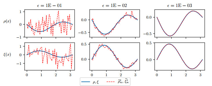
The main goal of this work is to study a regularization method to reconstruct the solution of the backward non-linear hyperbolic equation $ u_{tt} + \alpha\Delta^2u_t +\beta \Delta ^2u = \mathcal{F}(x, t, u) $ come with the input data are blurred by random Gaussian white noise. We first prove that the considered problem is ill-posed (in the sense of Hadamard), i.e., the solution does not depend continuously on the data. Then we propose the Fourier truncation method for stabilizing the ill-posed problem. Base on some priori assumptions for the true solution we derive the error and a convergence rate between a mild solution and its regularized solutions. Also, a numerical example is provided to confirm the efficiency of theoretical results.
- wave equations,
- hyperbolic equations,
- Gaussian white noise,
- random noise,
- regularized solution,
- ill-posed
Citation: Phuong Nguyen Duc, Erkan Nane, Omid Nikan, Nguyen Anh Tuan. Approximation of the initial value for damped nonlinear hyperbolic equations with random Gaussian white noise on the measurements[J]. AIMS Mathematics, 2022, 7(7): 12620-12634. doi: 10.3934/math.2022698

Related Papers:

Abstract

The main goal of this work is to study a regularization method to reconstruct the solution of the backward non-linear hyperbolic equation $ u_{tt} + \alpha\Delta^2u_t +\beta \Delta ^2u = \mathcal{F}(x, t, u) $ come with the input data are blurred by random Gaussian white noise. We first prove that the considered problem is ill-posed (in the sense of Hadamard), i.e., the solution does not depend continuously on the data. Then we propose the Fourier truncation method for stabilizing the ill-posed problem. Base on some priori assumptions for the true solution we derive the error and a convergence rate between a mild solution and its regularized solutions. Also, a numerical example is provided to confirm the efficiency of theoretical results.

References

[1]	M. Aassila, A. Guesmia, Energy decay for a damped nonlinear hyperbolic equation, Appl. Math. Lett., 12 (1999), 49–52. https://doi.org/10.1016/S0893-9659(98)00171-2 doi: 10.1016/S0893-9659(98)00171-2
[2]	G. Chen, F. Da, Blow-up of solution of Cauchy problem for three-dimensional damped nonlinear hyperbolic equation, Nonlinear Anal. Theor., 71 (2009), 358–372. https://doi.org/10.1016/j.na.2008.10.132 doi: 10.1016/j.na.2008.10.132
[3]	P.-L. Chow, I. A. Ibragimov, R. Z. Khasminskii, Statistical approach to some ill-posed problems for linear partial differential equations, Probab. Theory Relat. Fields, 113 (1999), 421–441. https://doi.org/10.1007/s004400050212 doi: 10.1007/s004400050212
[4]	C. Cao, M. A. Rammaha, E. S. Titi, Gevrey regularity for nonlinear analytic parabolic equations on the sphere, J. Dyn. Differ. Equ., 12 (2000), 411–433. https://doi.org/10.1023/A:1009072526324 doi: 10.1023/A:1009072526324
[5]	G. Chen, Y. Wang, Z. Zhao, Blow-up of solution of an initial boundary value problem for a damped nonlinear hyperbolic equation, Appl. Math. Lett., 17 (2004), 491–497. https://doi.org/10.1016/S0893-9659(04)90116-4 doi: 10.1016/S0893-9659(04)90116-4
[6]	C. Foias, R. Temam, Gevrey class regularity for the solutions of the Navier-Stokes equations, J. Funct. Anal., 87 (1989), 359–369. https://doi.org/10.1016/0022-1236(89)90015-3 doi: 10.1016/0022-1236(89)90015-3
[7]	L. Hörmander, Linear partial differential operators, Berlin, Heidelberg: Springer, 1963. https://doi.org/10.1007/978-3-642-46175-0
[8]	A. Imani, D. Ganji, H. B. Rokni, H. Latifizadeh, E. Hesameddini, M. H. Rafiee, Approximate traveling wave solution for shallow water wave equation, Appl. Math. Model., 36 (2012), 1550–1557. https://doi.org/10.1016/j.apm.2011.09.030 doi: 10.1016/j.apm.2011.09.030
[9]	W. Liu, K. Chen, Existence and general decay for nondissipative hyperbolic differential inclusions with acoustic/memory boundary conditions, Math. Nachr., 289 (2016), 300–320. https://doi.org/10.1002/mana.201400343 doi: 10.1002/mana.201400343
[10]	J. C. Maxwell, Ⅷ. A dynamical theory of the electromagnetic field, Phil. Trans. R. Soc., 155 (1865), 459–512. https://doi.org/10.1098/rstl.1865.0008 doi: 10.1098/rstl.1865.0008
[11]	P. Mathé, S. V. Pereverzev, Optimal discretization of inverse problems in hilbert scales. Regularization and self-regularization of projection methods, SIAM J. Numer. Anal., 38 (2001), 1999–2021. https://doi.org/10.1137/S003614299936175X doi: 10.1137/S003614299936175X
[12]	D. Picard, G. Kerkyacharian, Estimation in inverse problems and second-generation wavelets, In: Proceedings of the international congress of mathematicians, European Mathematical Society Publishing House, Madrid, August 22–30, 2006,713–739. https://doi.org/10.4171/022-3/37
[13]	A. D. Pierce, Acoustics: an introduction to its physical principles and applications, Cham: Springer, 2019. https://doi.org/10.1007/978-3-030-11214-1
[14]	N. D. Phuong, N. H. Tuan, D. Baleanu, T. B. Ngoc, On Cauchy problem for nonlinear fractional differential equation with random discrete data, Appl. Math. Comput., 362 (2019), 124458. https://doi.org/10.1016/j.amc.2019.05.029 doi: 10.1016/j.amc.2019.05.029
[15]	C. Song, Z. Yang, Existence and nonexistence of global solutions to the cauchy problem for a nonlinear beam equation, Math. Method. Appl. Sci., 33 (2010), 563–575. https://doi.org/10.1002/mma.1175 doi: 10.1002/mma.1175
[16]	N. H. Tuan, V. V. Au, N. H. Can, Regularization of initial inverse problem for strongly damped wave equation, Appl. Anal., 97 (2018), 69–88. https://doi.org/10.1080/00036811.2017.1359560 doi: 10.1080/00036811.2017.1359560
[17]	N. H. Tuan, D. Baleanu, T. N. Thach, D. O'Regan, N. H. Can, Final value problem for nonlinear time fractional reaction-diffusion equation with discrete data, J. Comput. Appl. Math., 376 (2020), 112883. https://doi.org/10.1016/j.cam.2020.112883 doi: 10.1016/j.cam.2020.112883
[18]	N. A. Triet, T. T. Binh, N. D. Phuong, D. Baleanu, N. H. Can, Recovering the initial value for a system of nonlocal diffusion equations with random noise on the measurements, Math. Method. Appl. Sci., 44 (2021), 5188–5209. https://doi.org/10.1002/mma.7102 doi: 10.1002/mma.7102
[19]	N. H. Tuan, D. V. Nguyen, V. V. Au, D. Lesnic, Recovering the initial distribution for strongly damped wave equation, Appl. Math. Lett., 73 (2017), 69–77. https://doi.org/10.1016/j.aml.2017.04.014 doi: 10.1016/j.aml.2017.04.014
[20]	N. H. Tuan, E. Nane, D. O'Regan, N. D. Phuong, Approximation of mild solutions of a semilinear fractional differential equation with random noise, Proc. Amer. Math. Soc., 148 (2020), 3339–3357. https://doi.org/10.1090/proc/15029 doi: 10.1090/proc/15029
[21]	G. F. Wheeler, W. P. Crummett, The vibrating string controversy, Am. J. Phys., 55 (1987), 33–37. https://doi.org/10.1119/1.15311 doi: 10.1119/1.15311
[22]	G. A. Zou, B. Wang, Stochastic Burgers' equation with fractional derivative driven by multiplicative noise, Comput. Math. Appl., 74 (2017), 3195–3208. https://doi.org/10.1016/j.camwa.2017.08.023 doi: 10.1016/j.camwa.2017.08.023

Reader Comments

Your name:*

Email:*
© 2022 the Author(s), licensee AIMS Press. This is an open access article distributed under the terms of the Creative Commons Attribution License (http://creativecommons.org/licenses/by/4.0)