White noise estimation for linear discrete fractional order system

Yantong Mu; Huihong Zhao; Zhifang Li; Yantong Mu; Huihong Zhao; Zhifang Li

doi:10.3934/math.2022558

AIMS Mathematics

2022, Volume 7, Issue 6: 10009-10023. doi: 10.3934/math.2022558

Previous Article Next Article

Research article

White noise estimation for linear discrete fractional order system

School of Mathematics and Statistics, Qilu University of Technology (Shandong Academy of Sciences), Jinan 250353, China

Received: 17 January 2022 Revised: 27 February 2022 Accepted: 07 March 2022 Published: 21 March 2022
MSC : 93C55, 93E11

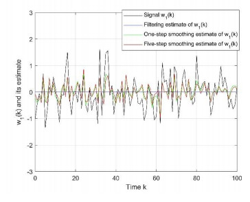
The process white noise (PWN) and observation white noise (OWN) estimation problem for linear discrete fractional order systems (LDFOS) is addressed in this study. By using the Grünwald-Letnikov (G-L) operator as a definition of the discrete fractional calculus (DFC), LDFOS is transformed into a class of linear discrete time-delay systems. However, it is different from the general time-delay system, in which the time-delay part is the cumulative sum from time 0 to the previous time. Based on the orthogonal projection theorem, a suboptimal one-step predictor of LDFOS is designed. Due to the existence of cumulative sum time-delay in system, the Riccati equation has one more cumulative sum state error variance term, which is different from the classical Kalman filter (KF). Moreover, using innovation analysis technology, the filtering and fixed-lag smoothing estimators of PWN and OWN in the form of noise orthogonal projection gain matrices are derived. Finally, two simulation examples are given to verify the effectiveness of PWN and OWN estimators.
- white noise,
- fractional order system,
- one-step predictor,
- filtering,
- fixed-lag smoothing
Citation: Yantong Mu, Huihong Zhao, Zhifang Li. White noise estimation for linear discrete fractional order system[J]. AIMS Mathematics, 2022, 7(6): 10009-10023. doi: 10.3934/math.2022558

Related Papers:

Abstract

The process white noise (PWN) and observation white noise (OWN) estimation problem for linear discrete fractional order systems (LDFOS) is addressed in this study. By using the Grünwald-Letnikov (G-L) operator as a definition of the discrete fractional calculus (DFC), LDFOS is transformed into a class of linear discrete time-delay systems. However, it is different from the general time-delay system, in which the time-delay part is the cumulative sum from time 0 to the previous time. Based on the orthogonal projection theorem, a suboptimal one-step predictor of LDFOS is designed. Due to the existence of cumulative sum time-delay in system, the Riccati equation has one more cumulative sum state error variance term, which is different from the classical Kalman filter (KF). Moreover, using innovation analysis technology, the filtering and fixed-lag smoothing estimators of PWN and OWN in the form of noise orthogonal projection gain matrices are derived. Finally, two simulation examples are given to verify the effectiveness of PWN and OWN estimators.

References

[1]	A. Ahlén, M. Sternad, Optimal deconvolution based on polynomial methods, IEEE Transactions on Acoustics, Speech, and Signal Processing, 37 (1989), 217‒226. http://dx.doi.org/10.1109/29.21684 doi: 10.1109/29.21684
[2]	J. Mendel, White-noise estimators for seismic data processing in oil exploration, IEEE T. Automat. Contr., 22 (1977), 694‒706. http://dx.doi.org/10.1109/TAC.1977.1101597 doi: 10.1109/TAC.1977.1101597
[3]	Y. Wang, Y. Zheng, Kalman filter based fault diagnosis of networked control system with white noise, J. Control Theory Appl., 1 (2005), 55‒59. http://dx.doi.org/10.1007/s11768-005-0061-y doi: 10.1007/s11768-005-0061-y
[4]	R. Singh, H. Parthasarathy, J. Singh, Time-varying image restoration using extended Kalman filter, Proceedings of 15th IEEE India Council International Conference (INDICON), 2018, 1‒6. http://dx.doi.org/10.1109/INDICON45594.2018.8986978 doi: 10.1109/INDICON45594.2018.8986978
[5]	J. Jiang, Y. Li, P. Zhang, Q. Hao, X. Ma, Y. Fan, Adaptive acoustic masking based on spectral envelope, Proceedings of International Conference on Audio, Language and Image Processing (ICALIP), 2016,442‒446. http://dx.doi.org/10.1109/ICALIP.2016.7846619 doi: 10.1109/ICALIP.2016.7846619
[6]	F. Atici, P. Eloe, Initial value problems in discrete fractional calculus, P. Am. Math. Soc., 137 (2009), 981‒989. http://dx.doi.org/10.1090/s0002-9939-08-09626-3 doi: 10.1090/s0002-9939-08-09626-3
[7]	L. Huang, G. Wu, D. Baleanu, H. Wang, Discrete fractional calculus for interval-valued systems, Fuzzy Set. Syst., 404 (2021), 141‒158. http://dx.doi.org/10.1016/j.fss.2020.04.008 doi: 10.1016/j.fss.2020.04.008
[8]	G. Wu, M. Cankaya, S. Banerjee, Fractional q-deformed chaotic maps: a weight function approach, Chaos, 12 (2020), 112106. http://dx.doi.org/10.1063/5.0030973 doi: 10.1063/5.0030973
[9]	D. Sierociuk, A. Dzielinski, Fractional Kalman filter algorithm for the states, parameters and order of fractional system estimation, Int. J. Appl. Math. Comput. Sci., 16 (2006), 129‒140.
[10]	J. Zarei, M. Tabatabaei, R. Razavi-Far, M. Saif, Fractional order unknown input filter design for fault detection of discrete linear systems, Proceedings of IECON - 43rd Annual Conference of the IEEE Industrial Electronics Society, 2017, 4333‒4338. http://dx.doi.org/10.1109/IECON.2017.8216745 doi: 10.1109/IECON.2017.8216745
[11]	H. Sadeghian, H. Salarieh, A. Alasty, A. Meghdari, On the general Kalman filter for discrete time stochastic fractional systems, Mechatronics, 23 (2013), 764‒771. http://dx.doi.org/10.1016/J.MECHATRONICS.2013.02.006 doi: 10.1016/J.MECHATRONICS.2013.02.006
[12]	D. Sierociuk, I. Tejado, B. Vinagre, Improved fractional Kalman filter and its application to estimation over lossy networks, Signal Process., 91 (2011), 542‒552. http://dx.doi.org/10.1016/j.sigpro.2010.03.014 doi: 10.1016/j.sigpro.2010.03.014
[13]	R. Ram, M. Mohanty, Application of fractional calculus in speech enhancement: a novel approach, Proceedings of 2nd International Conference on Data Science and Business Analytics (ICDSBA), 2018,123‒126. http://dx.doi.org/10.1109/ICDSBA.2018.00029 doi: 10.1109/ICDSBA.2018.00029
[14]	X. Wu, Y. Sun, Z. Lu, Z. Wei, M. Ni, W. Yu, A modified Kalman filter algorithm for fractional system under Lévy noises, J. Franklin. I., 352 (2015), 1963‒1978. http://dx.doi.org/10.1016/j.jfranklin.2015.02.008 doi: 10.1016/j.jfranklin.2015.02.008
[15]	J. Wang, L. Zhang, J. Mao, J. Zhou, D. Xu, Fractional order equivalent circuit model and SOC estimation of supercapacitors for use in HESS, IEEE Access, 7 (2019), 52565‒52572. http://dx.doi.org/10.1109/ACCESS.2019.2912221 doi: 10.1109/ACCESS.2019.2912221
[16]	G. Jin, L. Li, Y. Xu, M. Hu, C. Fu, D. Qin, Comparison of SOC estimation between the integer-order model and fractional-order model under different operating conditions, Energies, 13 (2020), 1785. http://dx.doi.org/10.3390/en13071785 doi: 10.3390/en13071785
[17]	Q. Zhu, M. Xu, W. Liu, M. Zheng, A state of charge estimation method for lithium-ion batteries based on fractional order adaptive extended kalman filter, Energy, 187 (2019), 115880. http://dx.doi.org/10.1016/J.ENERGY.2019.115880 doi: 10.1016/J.ENERGY.2019.115880
[18]	M. Xu, Q. Zhu, M. Zheng, A state of charge estimation approach based on fractional order adaptive extended Kalman filter for lithium-ion batteries, Proceedings of IEEE 7th Data Driven Control and Learning Systems Conference (DDCLS), 2018,271‒276. http://dx.doi.org/10.1109/DDCLS.2018.8516091 doi: 10.1109/DDCLS.2018.8516091
[19]	T. Raïssi, M. Aoun, On robust pseudo state estimation of fractional order systems, In: Lecture notes in control and information sciences, Switzerland: Springer, 2016, 97‒111. http://dx.doi.org/10.1007/978-3-319-54211-9_8
[20]	G. Wu, M. Luo, L. Huang, S. Banerjee, Short memory fractional differential equations for new neural network and memristor design, Nonlinear Dyn., 100 (2020), 3611‒3623. http://dx.doi.org/10.1007/s11071-020-05572-z doi: 10.1007/s11071-020-05572-z
[21]	H. Dehestani, Y. Ordokhani, M. Razzaghi, Fractional-order Bessel wavelet functions for solving variable order fractional optimal control problems with estimation error, Int. J. Syst. Sci., 51 (2020), 1032‒1052. http://dx.doi.org/10.1080/00207721.2020.1746980 doi: 10.1080/00207721.2020.1746980
[22]	H. Li, State estimation for fractional-order complex dynamical networks with linear fractional parametric uncertainty, Abstr. Appl. Anal., 2013 (2013), 178718. http://dx.doi.org/10.1155/2013/178718 doi: 10.1155/2013/178718
[23]	T. Abdeljawad, S. Banerjee, G. Wu, Discrete tempered fractional calculus for new chaotic systems with short memory and image encryption, Optik, 218 (2020), 163698. http://dx.doi.org/10.1016/j.ijleo.2019.163698 doi: 10.1016/j.ijleo.2019.163698
[24]	D. Idiou, A. Charef, A. Djouambi, Linear fractional order system identification using adjustable fractional order differentiator, IET Signal Process., 8 (2014), 398‒409. http://dx.doi.org/10.1049/iet-spr.2013.0002 doi: 10.1049/iet-spr.2013.0002

Reader Comments

Your name:*

Email:*
© 2022 the Author(s), licensee AIMS Press. This is an open access article distributed under the terms of the Creative Commons Attribution License (http://creativecommons.org/licenses/by/4.0)