Numerical solution of stochastic and fractional competition model in Caputo derivative using Newton method

Meihua Huang; Pongsakorn Sunthrayuth; Amjad Ali Pasha; Muhammad Altaf Khan; Meihua Huang; Pongsakorn Sunthrayuth; Amjad Ali Pasha; Muhammad Altaf Khan

doi:10.3934/math.2022498

AIMS Mathematics

2022, Volume 7, Issue 5: 8933-8952. doi: 10.3934/math.2022498

Previous Article Next Article

Research article Special Issues

Numerical solution of stochastic and fractional competition model in Caputo derivative using Newton method

1.
School of Marxism Studies (Department of Public Education), Nantong Open University, Nantong, Jiangsu, China
2.
Department of Mathematics and Computer Science, Faculty of Science and Technology, Rajamangala University of Technology Thanyaburi (RMUTT), Thanyaburi, Pathumthani, 12110, Thailand
3.
Aerospace Engineering Department, King Abdulaziz University, Jeddah 21589, Saudi Arabia
4.
Institute for Groundwater Studies, Faculty of Natural and Agricultural Sciences, University of the Free State, South Africa

Received: 06 January 2022 Revised: 18 February 2022 Accepted: 27 February 2022 Published: 07 March 2022
MSC : 34A08, 37N30

Many useful numerical algorithms of the numerical solution are proposed due to the increasing interest of the researchers in fractional calculus. A new discretization of the competition model for the real statistical data of banking finance for the years 2004–2014 is presented. We use a novel numerical method that is more reliable and accurate which is introduced recently for the solution of ordinary differential equations numerically. We apply this approach to solve our model for the case of Caputo derivative. We apply the Caputo derivative on the competition system and obtain its numerical results. For the numerical solution of the competition model, we use the Newton polynomial approach and present in detail a novel numerical procedure. We utilize the numerical procedure and present various numerical results in the form of graphics. A comparison of the present method versus the predictor corrector method is presented, which shows the same solution behavior to the Newton Polynomial approach. We also suggest that the real data versus model provide good fitting for both the data for the fractional-order parameter value $ \rho = 0.7 $. Some more values of $ \rho $ are used to obtain graphical results. We also check the model in the stochastic version and show the model behaves well when fitting to the data.
- Caputo derivative,
- Newton polynomial approach,
- real data 2004–2014,
- numerical algorithm,
- stochastic version
Citation: Meihua Huang, Pongsakorn Sunthrayuth, Amjad Ali Pasha, Muhammad Altaf Khan. Numerical solution of stochastic and fractional competition model in Caputo derivative using Newton method[J]. AIMS Mathematics, 2022, 7(5): 8933-8952. doi: 10.3934/math.2022498

Related Papers:

Abstract

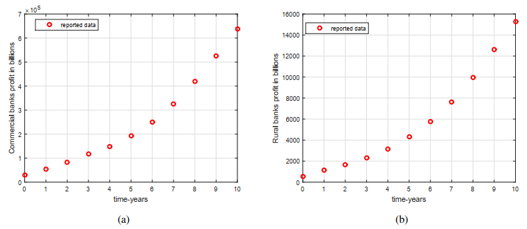
Many useful numerical algorithms of the numerical solution are proposed due to the increasing interest of the researchers in fractional calculus. A new discretization of the competition model for the real statistical data of banking finance for the years 2004–2014 is presented. We use a novel numerical method that is more reliable and accurate which is introduced recently for the solution of ordinary differential equations numerically. We apply this approach to solve our model for the case of Caputo derivative. We apply the Caputo derivative on the competition system and obtain its numerical results. For the numerical solution of the competition model, we use the Newton polynomial approach and present in detail a novel numerical procedure. We utilize the numerical procedure and present various numerical results in the form of graphics. A comparison of the present method versus the predictor corrector method is presented, which shows the same solution behavior to the Newton Polynomial approach. We also suggest that the real data versus model provide good fitting for both the data for the fractional-order parameter value $ \rho = 0.7 $. Some more values of $ \rho $ are used to obtain graphical results. We also check the model in the stochastic version and show the model behaves well when fitting to the data.

References

[1]	X. P. Li, Y. Wang, M. A. Khan, M. Y. Alshahrani, T. Muhammad, A dynamical study of SARS-COV-2: A study of third wave, Res. Phys., 29 (2021), 1–6. https://doi.org/10.1016/j.rinp.2021.104705 doi: 10.1016/j.rinp.2021.104705
[2]	Z. H. Shen, Y. M. Chu, M. A. Khan, S. Muhammad, O. A. AlHartomy, M. Higazy, Mathematical modeling and optimal control of the COVID-19 dynamics, Res. Phy., 31 (2021), 1–9. https://doi.org/10.1016/j.rinp.2021.105028 doi: 10.1016/j.rinp.2021.105028
[3]	X. P. Li, N. Gul, M. A. Khan, R. Bilal, A. Ali, M. Y. Alshahrani, et al., A new Hepatitis B model in light of asymptomatic carriers and vaccination study through Atangana-Baleanu derivative, Res. Phys., 29 (2021), 104603. https://doi.org/10.1016/j.rinp.2021.104603 doi: 10.1016/j.rinp.2021.104603
[4]	P. Y. Xiong, M. I. Khan, R. J. P. Gowda, R. N. Kumar, B. C. Prasannakumara, Y. M. Chu, Comparative analysis of (Zinc ferrite, Nickel Zinc ferrite) hybrid nanofluids slip flow with entropy generation, Mod. Phys. Lett. B, 35 (2021), 1–22.
[5]	P. Y. Xiong, A. Hamid, Y. M. Chu, M. I. Khan, R. J. P. Gowda, R. N. Kumar, et al., Dynamics of multiple solutions of Darcy-Forchheimer saturated flow of Cross nanofluid by a vertical thin needle point, Eur. Phys. J. Plus, 136 (2021), 1–22. https://doi.org/10.1140/epjp/s13360-021-01294-2 doi: 10.1140/epjp/s13360-021-01294-2
[6]	Laws of the republic indonesia number 10 year 1998 about amendment to law number 7 of 1992 concerning banking. Available from: https://www.global-regulation.com/translation/indonesia/7224941/act-no.-10-of-1998.html.
[7]	S. Arbi, Lembaga perbankan keuangan dan pembiayaan, Yogyakarta: BPFE, 2013.
[8]	S. Iskandar, Bank dan lembaga keuangan lainnya, Jakarta: Penerbit, 2013.
[9]	OJK, Statistik Perbankan Indonesia, 2004–2014. Available from: http://www.ojk.go.id/datastatistikperbankan-indonesia.
[10]	A. Hastings, Population biology: Concepts and models, Springer Science & Business Media, 2013.
[11]	J. Kim, D. J. Lee, J. Ahn, A dynamic competition analysis on the korean mobile phone market using competitive diffusion model, Comput. Ind. Eng., 51 (2006), 174–182. https://doi.org/10.1016/j.cie.2006.07.009 doi: 10.1016/j.cie.2006.07.009
[12]	S. A. Morris, D. Pratt, Analysis of the lotka-volterra competition equations as a technological substitution model, Technol. Forecast. Soc., 70 (2003), 103–133. https://doi.org/10.1016/S0040-1625(01)00185-8 doi: 10.1016/S0040-1625(01)00185-8
[13]	S. J. Lee, D. J. Lee, H. S. Oh, Technological forecasting at the korean stock market: A dynamic competition analysis using lotka-volterra model, Technol. Forecast. Soc., 72 (2005), 1044–1057. https://doi.org/10.1016/j.techfore.2002.11.001 doi: 10.1016/j.techfore.2002.11.001
[14]	C. Michalakelis, C. Christodoulos, D. Varoutas, T. Sphicopoulos, Dynamic estimation of markets exhibiting a prey-predator behavior, Expert Syst. Appl., 39 (2012), 7690–7700. https://doi.org/10.1016/j.eswa.2012.01.049 doi: 10.1016/j.eswa.2012.01.049
[15]	S. Lakka, C. Michalakelis, D. Varoutas, D. Martakos, Competitive dynamics in the operating systems market: Modeling and policy implications, Technol. Forecast. Soc., 80 (2013), 88–105. https://doi.org/10.1016/j.techfore.2012.06.011 doi: 10.1016/j.techfore.2012.06.011
[16]	C. A. Comes, Banking system: Three level lotka-volterra model, Proc. Econ. Financ., 3 (2012), 251–255. https://doi.org/10.1016/S2212-5671(12)00148-7 doi: 10.1016/S2212-5671(12)00148-7
[17]	Fatmawati, M. A. Khan, M. Azizah, Windarto, S. Ullah, A fractional model for the dynamics of competition between commercial and rural banks in Indonesia, Chaos Soliton. Fract., 122 (2019), 32–46. https://doi.org/10.1016/j.chaos.2019.02.009 doi: 10.1016/j.chaos.2019.02.009
[18]	W. Wang, M. A. Khan, Fatmawati, P. Kumam, P. Thounthong, A comparison study of bank data in fractional calculus, Chaos Soliton. Fract., 126 (2019), 369–384. https://doi.org/10.1016/j.chaos.2019.07.025 doi: 10.1016/j.chaos.2019.07.025
[19]	Z. F. Li, Z. Liu, M. A. Khan, Fractional investigation of bank data with fractal-fractional Caputo derivative, Chaos Soliton. Fract., 131 (2020), 109528. https://doi.org/10.1016/j.chaos.2019.109528 doi: 10.1016/j.chaos.2019.109528
[20]	W. Wang, M. A. Khan, Analysis and numerical simulation of fractional model of bank data with fractal-fractional Atangana-Baleanu derivative, J. Comput. Appl. Math., 369 (2020), 112646. https://doi.org/10.1016/j.cam.2019.112646 doi: 10.1016/j.cam.2019.112646
[21]	M. A. Khan, M. Azizah, S. Ullah, A fractional model for the dynamics of competition between commercial and rural banks in indonesia, Chaos Soliton. Fract., 122 (2019), 32–46. https://doi.org/10.1016/j.chaos.2019.02.009 doi: 10.1016/j.chaos.2019.02.009
[22]	S. Ullah, M. A. Khan, M. Farooq, A fractional model for the dynamics of tb virus, Chaos Soliton. Fract., 116 (2018), 63–71. https://doi.org/10.1016/j.chaos.2018.09.001 doi: 10.1016/j.chaos.2018.09.001
[23]	M. A. Khan, Fatmawati, A. Atangana, E. Alzahrani, The dynamics of COVID-19 with quarantined and isolation, Adv. Differ. Equ., 2020 (2020), 425. https://doi.org/10.1186/s13662-020-02882-9 doi: 10.1186/s13662-020-02882-9
[24]	Fatmawati, M. A. Khan, H. P. Odinsyah, Fractional model of HIV transmission with awareness effect, Chaos Soliton. Fract., 138 (2020), 109967. https://doi.org/10.1016/j.chaos.2020.109967 doi: 10.1016/j.chaos.2020.109967
[25]	A. Atangana, S. I. Araz, Atangana-Seda numerical scheme for Labyrinth attractor with new differential and integral operators, Fractals, 2020. https://doi.org/10.1142/S0218348X20400447
[26]	P. I, Fractional differential equations: An introduction to fractional derivatives, fractional differential equations, to methods of their solution and some of their applications, Academic Press, USA, 1998.
[27]	S. Das, P. Gupta, A mathematical model on fractional lotka-volterra equations, J. Theor. Biol., 277 (2011), 1–6. https://doi.org/10.1016/j.jtbi.2011.01.034 doi: 10.1016/j.jtbi.2011.01.034
[28]	M. A. Khan, Z. Hammouch, D. Baleanu, Modeling the dynamics of hepatitis E via the Caputo-Fabrizio derivative, Math. Model. Nat. Pheno., 14 (2019), 311. https://doi.org/10.1051/mmnp/2018074 doi: 10.1051/mmnp/2018074
[29]	M. A. Khan, S. Ullah, M. Farooq, A new fractional model for tuberculosis with relapse via atangana-baleanu derivative, Chaos Soliton. Fract., 116 (2018), 227–238. https://doi.org/10.1016/j.chaos.2018.09.039 doi: 10.1016/j.chaos.2018.09.039
[30]	F. Fatmawati, E. Shaiful, M. Utoyo, A fractional-order model for hiv dynamics in a two-sex population, Int. J. Math. Math. Sci., 2018 (2018). https://doi.org/10.1155/2018/6801475
[31]	A. Atangana, J. J. Nieto, Numerical solution for the model of rlc circuit via the fractional derivative without singular kernel, Adv. Mech. Eng., 7 (2015). https://doi.org/10.1177/1687814015613758
[32]	Y. Che, M. Y. A. Keir, Study on the training model of football movement trajectory drop point based on fractional differential equation, Appl. Math. Nonlinear Sci., 2021, 1–6. https://doi.org/10.2478/amns.2021.2.00095
[33]	S. Man, R. Yang, Educational reform informatisation based on fractional differential equation, Appl. Math. Nonlinear Sci., 2021, 1–10. https://doi.org/10.2478/amns.2021.2.00079
[34]	J. Gao, F. S. Alotaibi, R. T. Ismail, The model of sugar metabolism and exercise energy expenditure based on fractional linear regression equation, Appl. Math. Nonlinear Sci., 2021, 1–9. https://doi.org/10.2478/amns.2021.2.00026
[35]	N. Zhao, F. Yao, A. O. Khadidos, B. M. Muwafak, The impact of financial repression on manufacturing upgrade based on fractional Fourier transform and probability, Appl. Math. Nonlinear Sci., 2021, 1–11. https://doi.org/10.2478/amns.2021.2.00060
[36]	C. Li, N. Alhebaishi, M. A. Alhamami, Calculating university education model based on finite element fractional differential equations and macro-control analysis, Appl. Math. Nonlinear Sci., 2021, 1–10. https://doi.org/10.2478/amns.2021.2.00069
[37]	A. Zeb, E. Alzahrani, V. S. Erturk, G. Zaman, Mathematical model for coronavirus disease 2019 (COVID-19) containing isolation class, Biomed Res. Int., 2020 (2020). https://doi.org/10.1155/2020/3452402
[38]	Z. Zhang, A. Zeb, S. Hussain, E. Alzahrani, Dynamics of COVID-19 mathematical model with stochastic perturbation, Adv. Differ. Equ., 2020 (2020), 1–2. https://doi.org/10.1186/s13662-020-02909-1 doi: 10.1186/s13662-020-02909-1
[39]	S. Bushnaq, T. Saeed, D. F. Torres, A. Zeb, Control of COVID-19 dynamics through a fractional-order model, Alex. Eng. J., 60 (2021), 3587–3592. https://doi.org/10.1016/j.aej.2021.02.022 doi: 10.1016/j.aej.2021.02.022
[40]	Z. Zhang, A. Zeb, E. Alzahrani, S. Iqbal, Crowding effects on the dynamics of COVID-19 mathematical model, Adv. Differ. Equ., 2020 (2020), 1–3. https://doi.org/10.1186/s13662-020-03137-3 doi: 10.1186/s13662-020-03137-3
[41]	A. Din, Y. Li, A. Yousaf, A. I. Ali, Caputo type fractional operator applied to Hepatitis B system, Fractals, 2021. https://doi.org/10.1142/S0218348X22400230
[42]	A. Din, Y. Li, F. M. Khan, Z. U. Khan, P. Liu, On Analysis of fractional order mathematical model of Hepatitis B using Atangana-Baleanu Caputo (ABC) derivative, Fractals, 2021. https://doi.org/10.1142/S0218348X22400175
[43]	A. Din, A. Khan, A. Zeb, M. R. Sidi Ammi, M. Tilioua, D. F. Torres, Hybrid method for simulation of a fractional COVID-19 model with real case application, Axioms, 10 (2021), 290. https://doi.org/10.3390/axioms10040290 doi: 10.3390/axioms10040290
[44]	C. Xu, M. Liao, P. Li, S. Yuan, Impact of leakage delay on bifurcation in fractional-order complex-valued neural networks, Chaos Soliton. Fract., 142 (2021), 110535. https://doi.org/10.1016/j.chaos.2020.110535 doi: 10.1016/j.chaos.2020.110535
[45]	C. Xu, Z. Liu, L. Yao, C. Aouiti, Further exploration on bifurcation of fractional-order six-neuron bi-directional associative memory neural networks with multi-delays, Appl. Math. Comput., 410 (2021), 126458. https://doi.org/10.1016/j.amc.2021.126458 doi: 10.1016/j.amc.2021.126458
[46]	C. Xu, M. Liao, P. Li, Y. Guo, Q. Xiao, S. Yuan, Influence of multiple time delays on bifurcation of fractional-order neural networks, Appl. Math. Comput., 361 (2019), 565–582. https://doi.org/10.1016/j.amc.2019.05.057 doi: 10.1016/j.amc.2019.05.057
[47]	C. Xu, M. Liao, P. Li, Y. Guo, Z. Liu, Bifurcation properties for fractional order delayed BAM neural networks, Cogn. Comput., 13 (2021), 322–356. https://doi.org/10.1007/s12559-020-09782-w doi: 10.1007/s12559-020-09782-w
[48]	C. J. Xu, W. Zhang, C. Aouiti, Z. X. Liu, M. X. Liao, P. L. Li, Further investigation on bifurcation and their control of fractional-order BAM neural networks involving four neurons and multiple delays, Math. Meth. Appl. Sci., 2021, 75.
[49]	C. Xu, W. Zhang, Z. Liu, L. Yao, Delay-induced periodic oscillation for fractional-order neural networks with mixed delays, Neurocomputing, 2021. https://doi.org/10.1016/j.neucom.2021.11.079
[50]	OJK, Statistik Perbankan Indonesia 2004–2014.
[51]	A. Atangana, M. A. Khan, Modeling and analysis of competition model of bank data with fractal-fractional Caputo-Fabrizio operator, Alex. Eng. J., 159 (2020), 1985–1998. https://doi.org/10.1016/j.aej.2019.12.032 doi: 10.1016/j.aej.2019.12.032
[52]	A. Din, Y. Li, T. Khan, G. Zaman, Mathematical analysis of spread and control of the novel corona virus (COVID-19) in China, Chaos Soliton Fract., 141 (2020). https://doi.org/10.1016/j.chaos.2020.110286
[53]	A. Din, Y. Li, M. A. Shah, The complex dynamics of hepatitis B infected individuals with optimal control, J. Syst. Sci. Comput., 34 (2021), 1301–1323. https://doi.org/10.1007/s11424-021-0053-0 doi: 10.1007/s11424-021-0053-0
[54]	A. Din, T. Khan, Y. Li, H. Tahir, A. Khan, W. A. Khan, Mathematical analysis of dengue stochastic epidemic model, Result Phys., 20 (2021), 103719. https://doi.org/10.1016/j.rinp.2020.103719 doi: 10.1016/j.rinp.2020.103719
[55]	A. Din, Y. Li, The extinction and persistence of a stochastic model of drinking alcohol, Result Phys., 28 (2021), 104649. https://doi.org/10.1016/j.rinp.2021.104649 doi: 10.1016/j.rinp.2021.104649
[56]	A. Din, Y. Li, Stochastic optimal control for norovirus transmission dynamics by contaminated food and water, Chinese Phys. B, 2021. https://doi.org/10.1088/1674-1056/ac2f32
[57]	A. Atangana, Mathematical model of survival of fractional calculus, critics and their impact: How singular is our world? Adv. Differ. Equ., 2021 (2021), 1–59.
[58]	A. Atangana, S. I. Araz, Modeling third waves of Covid-19 spread with piecewise differential and integral operators: Turkey, Spain and Czechia, Result Phys., 29 (2021), 104694. https://doi.org/10.1016/j.rinp.2021.104694 doi: 10.1016/j.rinp.2021.104694
[59]	M. Caputo, Linear models of dissipation whose Q is almost frequency independent, part II, Geophys. J. Int., 13 (1967), 529–539.
[60]	A. Atangana, S. I. Araz, New numerical scheme with newton polynomial: Theory, methods, and applications, Academic Press, 2021.

Reader Comments

Your name:*

Email:*
© 2022 the Author(s), licensee AIMS Press. This is an open access article distributed under the terms of the Creative Commons Attribution License (http://creativecommons.org/licenses/by/4.0)