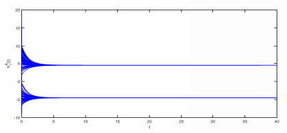
This paper addresses the problem of multi-stability analysis for fractional-order quaternion-valued neural networks (QVNNs) with time delay. Based on the geometrical properties of activation functions and intermediate value theorem, some conditions are derived for the existence of at least $ (2\mathcal{K}_p^R+1)^n, (2\mathcal{K}_p^I+1)^n, (2\mathcal{K}_p^J+1)^n, (2\mathcal{K}_p^K+1)^n $ equilibrium points, in which $ [(\mathcal{K}_p^R+1)]^n, [(\mathcal{K}_p^I+1)]^n, [(\mathcal{K}_p^J+1)]^n, [(\mathcal{K}_p^K+1)]^n $ of them are uniformly stable while the other equilibrium points become unstable. Thus the developed results show that the QVNNs can have more generalized properties than the real-valued neural networks (RVNNs) or complex-valued neural networks (CVNNs). Finally, two simulation results are given to illustrate the effectiveness and validity of our obtained theoretical results.
Citation: S. Kathiresan, Ardak Kashkynbayev, K. Janani, R. Rakkiyappan. Multi-stability analysis of fractional-order quaternion-valued neural networks with time delay[J]. AIMS Mathematics, 2022, 7(3): 3603-3629. doi: 10.3934/math.2022199
This paper addresses the problem of multi-stability analysis for fractional-order quaternion-valued neural networks (QVNNs) with time delay. Based on the geometrical properties of activation functions and intermediate value theorem, some conditions are derived for the existence of at least $ (2\mathcal{K}_p^R+1)^n, (2\mathcal{K}_p^I+1)^n, (2\mathcal{K}_p^J+1)^n, (2\mathcal{K}_p^K+1)^n $ equilibrium points, in which $ [(\mathcal{K}_p^R+1)]^n, [(\mathcal{K}_p^I+1)]^n, [(\mathcal{K}_p^J+1)]^n, [(\mathcal{K}_p^K+1)]^n $ of them are uniformly stable while the other equilibrium points become unstable. Thus the developed results show that the QVNNs can have more generalized properties than the real-valued neural networks (RVNNs) or complex-valued neural networks (CVNNs). Finally, two simulation results are given to illustrate the effectiveness and validity of our obtained theoretical results.

| [1] |
H. Wang, Y. Yu, G. Wen, S. Zhang, J. Yu, Global stability analysis of fractional-order Hopfield neural networks with time delay, Neurocomputing, 154 (2015), 15–23. doi: 10.1016/j.neucom.2014.12.031. doi: 10.1016/j.neucom.2014.12.031

|
| [2] |
R. Rakkiyappan, J. Cao, G. Velmurugan, Existence and uniform stability analysis of fractional-order complex-valued neural networks with time delays, IEEE Trans. Neural Netw. Learn. Syst., 26 (2015), 84–97. doi: 10.1109/TNNLS.2014.2311099. doi: 10.1109/TNNLS.2014.2311099
|
| [3] |
R. Rakkiyappan, K. Udhayakumar, G. Velmurugan, J. Cao, A. Alsaedi, Stability and Hopf bifurcation analysis of fractional-order complex-valued neural networks with time delays, Adv. Differ. Equ., 1 (2017), 1–25. doi: 10.1186/s13662-017-1266-3. doi: 10.1186/s13662-017-1266-3
|
| [4] |
G. Velmurugan, R. Rakkiyappan, J. Cao, Finite-time synchronization of fractional-order memristor-based neural networks with time delays, Neural Netw., 73 (2016), 36–46. doi: 10.1016/j.neunet.2015.09.012. doi: 10.1016/j.neunet.2015.09.012
|
| [5] |
A. Abdurahman, H. Jiang, Z. Teng, Finite-time synchronization for memristor-based neural networks with time-varying delays, Neural Netw., 69 (2015), 20–28. doi: 10.1016/j.neunet.2015.04.015. doi: 10.1016/j.neunet.2015.04.015
|
| [6] |
J. Cao, M. Xiao, Stability and Hopf bifurcation in a simplified BAM neural network with two time delays, IEEE Trans. Neural Netw. Learn. Syst., 18 (2007), 416–430. doi: 10.1109/TNN.2006.886358. doi: 10.1109/TNN.2006.886358
|
| [7] |
P. Liu, Z. Zeng, J. Wang, Multiple mittag–leffler stability of fractional-order recurrent neural networks, IEEE Trans. Syst. Man Cybern. Syst., 47 (2017), 2279–2288. doi: 10.1109/TSMC.2017.2651059. doi: 10.1109/TSMC.2017.2651059
|
| [8] |
A. Wu, Z. Zeng, Global Mittag-Leffler stabilization of fractional-order memristive neural networks, IEEE Trans. Neural Netw. Learn. Syst., 28 (2015), 206–217. doi: 10.1109/TNNLS.2015.2506738. doi: 10.1109/TNNLS.2015.2506738
|
| [9] |
X. Yang, C. Li, Q. Song, J. Chen, J. Huang, Global Mittag-Leffler stability and synchronization analysis of fractional-order quaternion-valued neural networks with linear threshold neurons, Neural Netw., 105 (2018), 88–103. doi: 10.1016/j.neunet.2018.04.015. doi: 10.1016/j.neunet.2018.04.015
|
| [10] |
Z. Sabir, M. A. Raja, M. Shoaib, J. G. Aguilar, FMNEICS: Fractional Meyer neuro-evolution-based intelligent computing solver for doubly singular multi-fractional order Lane–Emden system, Comput. Appl. Math., 39 (2020), 303. doi: 10.1007/s40314-020-01350-0. doi: 10.1007/s40314-020-01350-0
|
| [11] |
Z. Sabir, M. A. Raja, J. L. Guirao, M. Shoaib, A novel design of fractional Meyer wavelet neural networks with application to the nonlinear singular fractional Lane-Emden systems, Alex. Eng. J., 60 (2021), 2641–2659. doi: 10.1016/j.aej.2021.01.004. doi: 10.1016/j.aej.2021.01.004
|
| [12] |
Z. Sabir, M. A. Raja, J. L. Guirao, T. Saeed, Meyer wavelet neural networks to solve a novel design of fractional order pantograph Lane-Emden differential model, Chaos Soliton. Fract., 152 (2021), 111404. doi: 10.1016/j.chaos.2021.111404. doi: 10.1016/j.chaos.2021.111404
|
| [13] |
Z. Sabir, M. A. Raja, J. L. Guirao, T. Saeed, Solution of novel multi-fractional multi-singular Lane-Emden model using the designed FMNEICS, Neural Comput. Appl., 33 (2021), 17287–17302. doi: 10.1007/s00521-021-06318-7. doi: 10.1007/s00521-021-06318-7
|
| [14] |
Z. Sabir, M. A. Raja, D. Baleanu, Fractional Mayer Neuro-swarm heuristic solver for multi-fractional Order doubly singular model based on Lane-Emden equation, Fractals, 29 (2021), 2140017. doi: 10.1142/S0218348X2140017X. doi: 10.1142/S0218348X2140017X
|
| [15] |
A. Elsonbaty, Z. Sabir, R. Ramaswamy, W. Adel, Dynamical Analysis of a novel discrete fractional SITRS model for COVID-19, Fractals, 29 (2021), 2140035. doi: 10.1142/S0218348X21400351. doi: 10.1142/S0218348X21400351
|
| [16] |
E. Kaslik, I. R. Rǎdulescu, Dynamics of complex-valued fractional-order neural networks, Neural Netw., 89 (2017), 39–49. doi: 10.1016/j.neunet.2017.02.011. doi: 10.1016/j.neunet.2017.02.011
|
| [17] | I. Podlubny, Fractional differential equations, California: Academic Press, 1999. |
| [18] |
A. Aghili, Complete solution for the time fractional diffusion problem with mixed boundary conditions by operational method, Appl. Math. Nonlinear Sci., 6 (2020), 9–20. doi: 10.2478/AMNS.2020.2.00002. doi: 10.2478/AMNS.2020.2.00002
|
| [19] |
K. A. Touchent, Z. Hammouch, T. Mekkaoui, A modified invariant subspace method for solving partial differential equations with non-singular kernel fractional derivatives, Appl. Math. Nonlinear Sci., 5 (2020), 35–48. doi: 10.2478/amns.2020.2.00012. doi: 10.2478/amns.2020.2.00012
|
| [20] |
M. Onal, A. Esen, A Crank-Nicolson approximation for the time fractional Burgers equation, Appl. Math. Nonlinear Sci., 5 (2020), 177–184. doi: 10.2478/amns.2020.2.00023. doi: 10.2478/amns.2020.2.00023
|
| [21] |
A. O. Akdemir, E. Deniz, E. Yüksel, On Some integral inequalities via conformable fractional integrals, Appl. Math. Nonlinear Sci., 6 (2021), 489–498. doi: 10.2478/amns.2020.2.00071. doi: 10.2478/amns.2020.2.00071
|
| [22] | M. Gürbüz, C. Yildiz, Some new inequalities for convex functions via Riemann-Liouville fractional integrals, Appl. Math. Nonlinear Sci., 6 (2021) 537–544. doi: 10.2478/amns.2020.2.00015. |
| [23] |
S. Arik, Global asymptotic stability of a class of dynamical neural networks, IEEE Trans. Circuits Syst. I, Fundam. Theory Appl., 47 (2000), 568–571. doi: 10.1109/81.841858. doi: 10.1109/81.841858
|
| [24] |
H. Zhang, E. Fata, S. Sundaram, A notion of robustness in complex networks, IEEE T. Control Netw., 2 (2015), 310–320. doi: 10.1109/TCNS.2015.2413551. doi: 10.1109/TCNS.2015.2413551
|
| [25] |
Y. Huang, H. Zhang, Z. Wang, Multi-stability and multi-periodicity of delayed biderectional associative memory neural networks with discontinuous activation functions, Appl. Math. Comput., 219 (2012), 899–910. doi: 10.1016/j.amc.2012.06.068. doi: 10.1016/j.amc.2012.06.068
|
| [26] |
R. Rakkiyappan, G. Velmurugan, J. Cao, Finite-time stability analysis of fractional-order complex-valued memristor-based neural networks with time delays, Nonlinear Dynam., 78 (2014), 2823–2836. doi: 10.1007/s11071-014-1628-2. doi: 10.1007/s11071-014-1628-2
|
| [27] |
G. Velmurugan, R. Rakkiyappan, V. Vembarasan, J. Cao, A. Alsaedi, Dissipativity and stability analysis of fractional-order complex-valued neural networks with time delay, Neural Netw., 86 (2017), 42–53. doi: 10.1016/j.neunet.2016.10.010. doi: 10.1016/j.neunet.2016.10.010
|
| [28] |
X. Chen, Q. Song, Z. Li, Z. Zhao, Y. Liu, Stability analysis of continuous-time and discrete-time quaternion-valued neural networks with linear threshold neurons, IEEE Trans. Neural Netw. Learn. Syst., 29 (2018), 2769–2781. doi: 10.1109/TNNLS.2017.2704286. doi: 10.1109/TNNLS.2017.2704286
|
| [29] |
J. Hu, C. Zeng, J. Tan, Boundedness and periodicity for linear threshold discrete-time quaternion-valued neural network with time-delays, Neurocomputing, 267 (2017), 417–425. doi: 10.1016/j.neucom.2017.06.047. doi: 10.1016/j.neucom.2017.06.047
|
| [30] |
N. Li, W. X. Zheng, Passivity analysis for quaternion-valued memristor-based neural networks with time-varying delay, IEEE Trans. Neural Netw. Learn. Syst., 31 (2020), 639–650. doi: 10.1109/TNNLS.2019.2908755. doi: 10.1109/TNNLS.2019.2908755
|
| [31] |
Y. Liu, D. Zhang, J. Lu, Global exponential stability for quaternion-valued recurrent neural networks with time-varying delay, Nonlinear Dynam., 87 (2017), 553–565. doi: 10.1007/s11071-016-3060-2. doi: 10.1007/s11071-016-3060-2
|
| [32] |
Q. Song, X. Chen, Multistability analysis of quaternion-valued neural networks with time delay, IEEE Trans. Neural Netw. Learn. Syst., 29 (2017), 5430–5440. doi: 10.1109/TNNLS.2018.2801297. doi: 10.1109/TNNLS.2018.2801297
|
| [33] |
Y. Liu, D. Zhang, J. Lou, J. Lu, J. Cao, Stability analysis of quaternion-valued neural networks: Decomposition and direct approaches, IEEE Trans. Neural Netw. Learn. Syst., 29 (2018), 4201–4211. doi: 10.1109/TNNLS.2017.2755697. doi: 10.1109/TNNLS.2017.2755697
|
| [34] |
Y. Liu, D. Zhang, J. Lu, J. Cao, Global $\mu$-stability criteria for quaternion-valued neural networks with unbounded time-varying delays, Inform. Sciences, 360 (2016), 273–288. doi: 10.1016/j.ins.2016.04.033. doi: 10.1016/j.ins.2016.04.033
|
| [35] |
Z. Tu, J. Cao, A. Alsaedi, T. Hayat, Global dissipativity analysis for delayed quaternion-valued neural networks, Neural Netw., 89 (2017), 97–104. doi: 10.1016/j.neunet.2017.01.006. doi: 10.1016/j.neunet.2017.01.006
|
| [36] |
S. Zhang, Y. Yu, J. Yu, LMI conditions for global stability of fractional-order neural networks, IEEE Trans. Neural Netw. Learn. Syst., 28 (2017), 2423–2433. doi: 10.1109/TNNLS.2016.2574842. doi: 10.1109/TNNLS.2016.2574842
|
| [37] |
M. Ogura, V. M. Preciado, Stability of SIS Spreading Processes in Networks with Non-Markovian Transmission and Recovery, IEEE T. Control Netw., 7 (2020), 349–359. doi:10.1109/TCNS.2019.2905131. doi: 10.1109/TCNS.2019.2905131
|
| [38] |
F. Li, Stability of Boolean networks with delays using pinning control, IEEE T. Control Netw., 5 (2018), 179–185. doi: 10.1109/TCNS.2016.2585861. doi: 10.1109/TCNS.2016.2585861
|
| [39] |
F. Zhang, Z. Zeng, Multiple $\psi$-type stability of Cohen-Grossberg neural networks with unbounded time-varying delays, IEEE Trans. Syst. Man Cybern. Syst., 51 (2018), 521–531. doi: 10.1109/TSMC.2018.2876003. doi: 10.1109/TSMC.2018.2876003
|
| [40] |
F. Zhang, Z. Zeng, Multistability and instability analysis of recurrent neural networks with time-varying delays, Neural Netw., 97 (2018), 116–126. doi: 10.1016/j.neunet.2017.09.013. doi: 10.1016/j.neunet.2017.09.013
|
| [41] |
I. Karafyllis, M. Papageorgiou, Global exponential stability for discrete-time networks with applications to traffic networks, IEEE T. Control Netw., 2 (2015), 68–77. doi: 10.1109/TCNS.2014.2367364. doi: 10.1109/TCNS.2014.2367364
|
| [42] |
Z. Zeng, T. Huang, W. X. Zheng, Multistability of recurrent neural networks with time-varying delays and the piecewise linear activation function, IEEE Trans. Neural Netw. Learn. Syst., 21 (2010), 1371–1377. doi: 10.1109/TNN.2010.2054106. doi: 10.1109/TNN.2010.2054106
|
| [43] |
H. L. Li, L. Zhang, C. Hu, Y. L. Jiang, Z. Teng, Dynamical analysis of a fractional-order predator-prey model incorporating a prey refuge, J. Appl. Math. Comput., 54 (2017), 435–449. doi: 10.1007/s12190-016-1017-8. doi: 10.1007/s12190-016-1017-8
|
| [44] |
R. Wei, J. Cao, Fixed-time synchronization of quaternion-valued memristive neural networks with time delays, Neural Netw., 113 (2019), 1–10. doi: 10.1016/j.neunet.2019.01.014. doi: 10.1016/j.neunet.2019.01.014
|
| [45] |
H. L. Li, C. Hu, L. Zhang, H. Jiang, J. Cao, Non-separation method-based robust finite-time synchronization of uncertain fractional-order quaternion-valued neural networks, Appl. Math. Comput., 409 (2021), 126377. doi: 10.1016/j.amc.2021.126377. doi: 10.1016/j.amc.2021.126377
|
| [46] |
H. L. Li, H. Jiang, J. Cao, Global synchronization of fractional-order quaternion-valued neural networks with leakage and discrete delays, Neurocomputing, 385 (2020), 211–219. doi: 10.1016/j.neucom.2019.12.018. doi: 10.1016/j.neucom.2019.12.018
|
| [47] |
P. Liu, Z. Zeng, J. Wang, Multistability of recurrent neural networks with non-monotonic activation functions and unbounded time-varying delays, IEEE Trans. Neural Netw. Learn. Syst., 29 (2018), 3000–3010. doi: 10.1109/TSMC.2015.2461191. doi: 10.1109/TSMC.2015.2461191
|
| [48] |
Z. Zeng, W. X. Zheng. Multistability of neural networks with time-varying delays and concave-convex characteristics, IEEE Trans. Neural Netw. Learn. Syst., 23 (2012), 293–305. doi: 10.1109/TNNLS.2011.2179311. doi: 10.1109/TNNLS.2011.2179311
|
| [49] | A. Kilbas, H. Srivastava, J. Trujillo, Theory and applications of fractional differential equations, The Netherlands: Elsevier, 2006. |
| [50] |
I. Stamova, Global mittag-Leffler stability and synchronization of impulsive fractional-order neural networks with time-varying delays, Nonlinear Dynam., 77 (2014), 1251–1260. doi: 10.1007/s11071-014-1375-4. doi: 10.1007/s11071-014-1375-4
|
| [51] |
S. Tyagi, S. Abbas, M. Hafayed, Global Mittag-Leffler stability of complex valued fractional-order neural network with discrete and distributed delays, Rend. Circ. Mat. Palerm., 65 (2016), 485–505. doi: 10.1007/s12215-016-0248-8. doi: 10.1007/s12215-016-0248-8
|
| [52] | J. Zhang, Y. Xiang, N. Wang, Multiple Mittag-Leffler stability of fractional-order Cohen-Grossberg neural networks with non-monotonic piecewise linear activation functions, In: 2018 Tenth International Conference on Advanced Computational Intelligence (ICACI), 2018,520–527. doi: 10.1109/ICACI.2018.8377513. |
| [53] |
S. Zhang, Y. Yu, H. Wang, Mittag-Leffler stability of fractional-order Hopfield neural networks, Nonlinear Anal-Hybri., 16 (2015), 104–121. doi: 10.1016/j.nahs.2014.10.001. doi: 10.1016/j.nahs.2014.10.001
|


Figures(20)

S. Kathiresan, Ardak Kashkynbayev, K. Janani, R. Rakkiyappan. Multi-stability analysis of fractional-order quaternion-valued neural networks with time delay[J]. AIMS Mathematics, 2022, 7(3): 3603-3629. doi: 10.3934/math.2022199


 DownLoad: