A study of resonance Y-type multi-soliton solutions and soliton molecules for new (2+1)-dimensional nonlinear wave equations

Chun-Ku Kuo; Dipankar Kumar; Chieh-Ju Juan; Chun-Ku Kuo; Dipankar Kumar; Chieh-Ju Juan

doi:10.3934/math.20221136

AIMS Mathematics

2022, Volume 7, Issue 12: 20740-20751. doi: 10.3934/math.20221136

Previous Article Next Article

Research article

A study of resonance Y-type multi-soliton solutions and soliton molecules for new (2+1)-dimensional nonlinear wave equations

1.
Department of Aeronautics and Astronautics, Air Force Academy, Kaohsiung 820009, Taiwan
2.
Department of Mathematics, Bangabandhu Sheikh Mujibur Rahman Science and Technology University, Gopalganj 8100, Bangladesh
3.
Department of Aviation Management, Air Force Academy, Kaohsiung 820009, Taiwan

Received: 04 August 2022 Revised: 12 September 2022 Accepted: 19 September 2022 Published: 26 September 2022
MSC : 35C08, 35Q51, 37K40

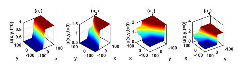
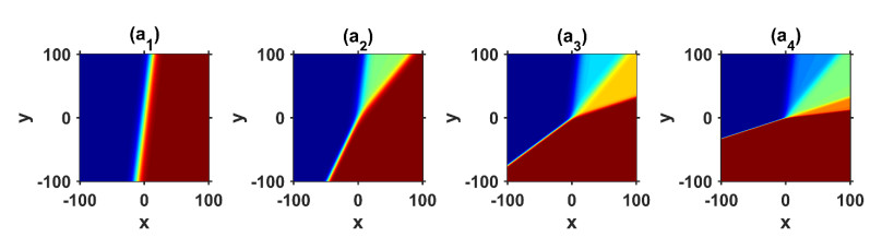
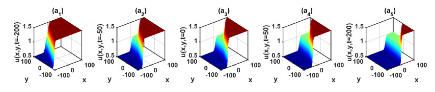
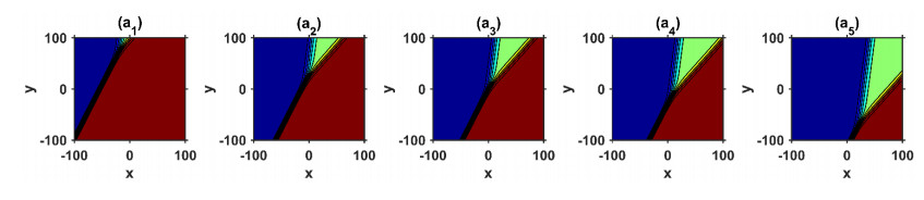
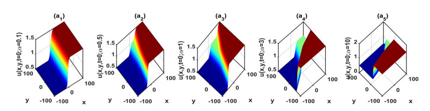
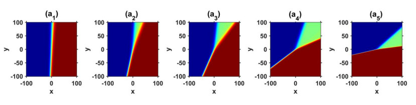
In this study, a fourth-order nonlinear wave equation with variable coefficients was investigated. Through appropriate choice of the free parameters and using the simplified linear superposition principle (LSP) and velocity resonance (VR), the examined equation can be considered as Hirota–Satsuma–Ito, Calogero–Bogoyavlenskii–Schiff and Jimbo–Miwa equations. The main objective of this study was to obtain novel resonant multi-soliton solutions and investigate inelastic interactions of traveling waves for the above-mentioned equation. Novel resonant multi-soliton solutions along with their essential conditions were obtained by using simplified LSP, and the conditions guaranteed the existence of resonant solitons. Furthermore, the obtained solutions were used to investigate the dynamic and fission behavior of Y-type multi-soliton waves. For an accurate investigation of physical phenomena, appropriate free parameters were chosen to ascertain the impact on the speed of traveling waves and the initiation time of fission. Three-dimensional and contour plots of the obtained solutions are presented in Figures 1–6. Additionally, two nonlinear equations were formulated and investigated using VR, and the related soliton molecules were simultaneously extracted. The reported resonant Y-type multi-soliton waves and equations are new and have not been previously investigated. They can be used to explain modeled physical phenomena and can provide information about dynamic behavior of shallow water waves.

Keywords:

simplified linear superposition principle,
velocity resonance,
soliton molecule,
resonant Y-type multi-soliton

Citation: Chun-Ku Kuo, Dipankar Kumar, Chieh-Ju Juan. A study of resonance Y-type multi-soliton solutions and soliton molecules for new (2+1)-dimensional nonlinear wave equations[J]. AIMS Mathematics, 2022, 7(12): 20740-20751. doi: 10.3934/math.20221136

Related Papers:

[1]	Keqiang Li, Shangjiu Wang . Multiple periodic solutions of nonlinear second order differential equations. AIMS Mathematics, 2023, 8(5): 11259-11269. doi: 10.3934/math.2023570
[2]	Wangjin Yao . Variational approach to non-instantaneous impulsive differential equations with $p$ -Laplacian operator. AIMS Mathematics, 2022, 7(9): 17269-17285. doi: 10.3934/math.2022951
[3]	Yuhua Long, Sha Li . Results on homoclinic solutions of a partial difference equation involving the mean curvature operator. AIMS Mathematics, 2025, 10(3): 6429-6447. doi: 10.3934/math.2025293
[4]	Liuyang Shao, Haibo Chen, Yicheng Pang, Yingmin Wang . Multiplicity of nontrivial solutions for a class of fractional Kirchhoff equations. AIMS Mathematics, 2024, 9(2): 4135-4160. doi: 10.3934/math.2024203
[5]	Minggang Xia, Xingyong Zhang, Danyang Kang, Cuiling Liu . Existence and concentration of nontrivial solutions for an elastic beam equation with local nonlinearity. AIMS Mathematics, 2022, 7(1): 579-605. doi: 10.3934/math.2022037
[6]	Andrey Muravnik . Nonclassical dynamical behavior of solutions of partial differential-difference equations. AIMS Mathematics, 2025, 10(1): 1842-1858. doi: 10.3934/math.2025085
[7]	D. Fernández-Ternero, E. Macías-Virgós, D. Mosquera-Lois, N. A. Scoville, J. A. Vilches . Fundamental theorems of Morse theory on posets. AIMS Mathematics, 2022, 7(8): 14922-14945. doi: 10.3934/math.2022818
[8]	Muhammad Sarwar, Aiman Mukheimer, Syed Khayyam Shah, Arshad Khan . Existence of solutions of fractal fractional partial differential equations through different contractions. AIMS Mathematics, 2024, 9(5): 12399-12411. doi: 10.3934/math.2024606
[9]	Yuhua Long . Existence of two homoclinic solutions for a nonperiodic difference equation with a perturbation. AIMS Mathematics, 2021, 6(5): 4786-4802. doi: 10.3934/math.2021281
[10]	Jun Lei, Hongmin Suo . Multiple solutions of Kirchhoff type equations involving Neumann conditions and critical growth. AIMS Mathematics, 2021, 6(4): 3821-3837. doi: 10.3934/math.2021227

Abstract

1. Introduction

1.1. Overview

Many physical phenomena, in the fields of sound and electrical waves, heat transfer, mechanics, and optics can be described through partial differential equations. Therefore, we can say that the study of mathematical physics depends primarily on the study of partial differential equations. During previous decades, many methods were developed to reduce and solve partial differential equations, including Symmetry method ^[1,2,3,4], scattering transformation ^[5], Tanh method ^[6], the homogeneous balance method ^[7], Aboodh transform decomposition method ^[8], ( $G^{\prime}/G$ , $1/G$ )-expansion method ^[9], Exp-function method ^[10], Generalized He's Exp-function method ^[11], Kudryashov method ^[12], and Generalized Kudryashov method ^[13]. Consider the nonlinear (2+1)-dimensional Date-Jimbo-Kashiwara-Miwa (DJKM) equation ^[14,15] in the following form:

$\begin{equation} \Phi_{xxxxy}+4\Phi_{xxy}\Phi_{x}+2\Phi_{xxx}\Phi_{y}+6\Phi_{xy}\Phi_{xx} +\Phi_{yyy}-2\Phi_{xxt} = 0, \end{equation}$

(1)

where $\Phi = \Phi(x, y, t).$ DJKM describes the wave diffusion of physical-quantity, and it has certain applications in plasma physics ^[16,17]. This equation was presented by Jimbo and Miwa as second formulas for Kadomtsev-Petviashvili hierarchy.

1.2. Related literatures

There is a wealth of literature related to this governing equation such as: Bibi and Ahmad ^[14] who employed the symmetry method to reduce the governing equation to another equation of lower order and obtained its exact solutions. The exp( $-\phi$ ( $\xi$ ))-Expansion Method was utilized by Sajid and Akram ^[14] for obtaining traveling wave solutions for Eq (1). Halder et al. ^[18] used the Lie symmetry analysis and singularity method to study one type of the governing equation. Wazwaz ^[19] studied the integrability of this equation and obtained multiple soliton solutions by using Painlevé analysis and Hirota's method. Akram et al. ^[16] applied the extended direct algebraic method to obtain exact solutions for the governing equation.

1.3. Main idea

The previous literature led us to determine the study of the governing equation to apply the Lie symmetry method and the Generalized Kudryashov method. Our main objective of this paper is to convert the governing equation to several distinct ordinary differential equations (ODE). We then solve the resulting ODEs to obtain exact and novel wave solutions for the governing equation. As a result, we can show the dynamic behavior of wave solutions in 2-D and 3-D plots.

2. Lie symmetry method

In this part, the Lie symmetry method ^[20,21,22] is used to deduce the similarity reductions for the governing equation, so the one-parameter Lie symmetry of infinitesimal variables is shown as follows:

$\begin{align*} t^{\ast} & = t+\varepsilon A(t,x,y,\Phi)+o(\varepsilon^{2}),\text{ }x^{\ast } = x+\varepsilon B(t,x,y,\Phi)+o(\varepsilon^{2}),\nonumber\\ y^{\ast} & = y+\varepsilon C(t,x,y,\Phi)+o(\varepsilon^{2}),\text{ } \Phi^{\ast} = \Phi+\varepsilon E(t,x,y,\Phi)+o(\varepsilon^{2}), \end{align*}$

(2)

where $\varepsilon$ is the one parameter Lie group, $A, \; B, \; C$ and $E$ are infinitesimal variables and $t, \; x$ and $y$ are independent variables of the function $\Phi.$

The vector generator $\chi$ is related to the above-mentioned group transformations which can be written as the following expression:

$\begin{equation} \chi = A\frac{\partial}{\partial t}+B\frac{\partial}{\partial x}+C\frac {\partial}{\partial y}+E\frac{\partial}{\partial\Phi}, \end{equation}$

(3)

when the following invariance condition is satisfied:

$\begin{equation} \Gamma^{(3)}(\Delta) = 0, \end{equation}$

(4)

where $\Delta$ represents Eq (1) and $\Gamma^{(3)}$ is the third order prolongation^[23,24] of the operator V

$\begin{align*} \Gamma^{(3)} & = \chi+E_{[x]}\frac{\partial}{\partial\Phi_{x}}+E_{[y]} \frac{\partial}{\partial\Phi_{y}}+E_{[xy]}\frac{\partial}{\partial\Phi_{xy} }+E_{[xxx]}\frac{\partial}{\partial\Phi_{xxx}}+E_{[xxy]}\frac{\partial }{\partial\Phi_{xxy}}\nonumber\\ & +E_{[xxt]}\frac{\partial\Phi}{\partial\Phi_{xxt}}+E_{[xxy]}\frac{\partial }{\partial\Phi_{xxy}}+E_{[xxxy]}\frac{\partial}{\partial\Phi_{xxxy}} +E_{[yyy]}\frac{\partial}{\partial\Phi_{yyy}}, \end{align*}$

(5)

where the components $E_{[x]}, E_{[xx]}, \; E_{[xyy]}, \; E_{[y]}, \; E_{[xy]}....$ can be determined from the following expressions:

$\begin{align*} E_{[x]} & = D_{x}E-\Phi_{t}D_{x}A-\Phi_{x}D_{x}B-\Phi_{y}D_{x}C,\nonumber\\ E_{[y]} & = D_{y}E-\Phi_{t}D_{y}A-\Phi_{x}D_{y}B-\Phi_{y}D_{y}C,\nonumber\\ \text{ }E_{[xx]} & = D_{x}E_{[x]}-\Phi_{xt}D_{x}A-\Phi_{xx}D_{x}B-\Phi _{xy}D_{x}C,\nonumber\\ \text{ }E_{[xy]} & = D_{y}E_{[x]}-\Phi_{xt}D_{y}A-\Phi_{xx}D_{y}B-\Phi _{xy}D_{y}C,\nonumber\\ \text{ }E_{[yy]} & = D_{y}E_{[y]}-\Phi_{xt}D_{y}A-\Phi_{xx}D_{y}B-\Phi _{xy}D_{y}C,\nonumber\\ E_{[xxxy]} & = D_{y}E_{[xxx]}-\Phi_{xxxt}D_{y}A-\Phi_{xxxx}D_{y}B-\Phi _{xxxy}D_{y}C. \end{align*}$

(6)

Substituting (1) into Eq (4), yields an identity components $A_{x}, A_{xx}, \; B_{t}, B_{x}, ....$ and adding the coefficients of $\Phi_{x, x, t}$ , $\Phi_{y, y, y}$ , ... and equating them to zero, then the infinitesimals $A, B, C$ and $E$ are obtained from the following equations:

$A_{x} = A_{y} = A_{\Phi} = 0,$

$B_{y} = B_{\Phi} = 0,B_{x} = \frac{1}{4}A_{t},$

$C_{x} = B_{\Phi} = 0,\text{ }C_{z} = \frac{1}{2}A_{t},$

$\begin{equation} E_{x} = \frac{-1}{2}C_{t},\text{ }E_{\Phi} = \frac{-1}{4}A_{t},\text{ }E_{y} = \frac{-1}{2}B_{t}. \end{equation}$

(7)

solving the system of Eq (7), we get

$\begin{align*} A & = g_{1}(t),\text{ }B = \frac{1}{4}g_{1}^{\prime}x+g_{3}(t),\text{ }C = \frac{1}{2}g_{1}^{\prime}y+g_{2}(t),\text{ }\nonumber\\ E & = \frac{-1}{4}g_{1}^{\prime}\Phi-\frac{1}{4}xyg_{1}^{\prime\prime} -yg_{2}^{\prime}-\frac{1}{2}xg_{3}^{\prime}+g_{4}(t). \end{align*}$

(8)

The vector field operator $V$ of Eq (8) can be presented as

$\begin{equation} V = V_{1}(c_{1})+V_{2}(c_{2})+V_{3}(c_{3})+V_{4}(c_{4}), \end{equation}$

(9)

where

$\begin{align*} V_{1} & = g_{1}(t)\left( \frac{\partial}{\partial t}+\frac{1}{4} x\frac{\partial}{\partial x}+\frac{1}{2}y\frac{\partial}{\partial y}-\frac {1}{4}\Phi\frac{\partial}{\partial\Phi}\right) -\frac{1}{4}xyg_{1} ^{\prime\prime}\frac{\partial}{\partial\Phi},\nonumber\\ V_{2} & = g_{2}(t)\frac{\partial}{\partial y}-y\alpha_{2}^{\prime} \frac{\partial}{\partial\Phi},\text{ }V_{3} = g_{3}(t)\frac{\partial }{\partial x}-\frac{1}{2}g_{3}^{\prime}\frac{\partial}{\partial\Phi},\text{ }V_{4} = g_{4}(t)\frac{\partial}{\partial\Phi}. \end{align*}$

(10)

The Lie-bracket $[V_{i}, V_{j}] = V_{i}V_{j}-V_{j}V_{i}$ is used for obtaining the commutator relations which are shown in Table 1, where

$\begin{align*} l_{1} & = g_{1}g_{2}^{\prime}-\frac{1}{2}g_{2}g_{1}^{\prime},\text{ } l_{2} = \frac{-1}{4}(g_{2}^{\prime}g_{1}^{\prime}+2g_{1}g_{2}^{\prime\prime }-g_{2}g_{1}^{\prime\prime})x,\nonumber\\ l_{3} & = g_{1}g_{3}^{\prime}-\frac{1}{4}g_{3}g_{1}^{\prime},\text{ } l_{4} = \frac{-1}{4}(g_{3}^{\prime}g_{1}^{\prime}+4g_{1}g_{3}^{\prime\prime }-g_{3}g_{1}^{\prime\prime})y,\nonumber\\ l_{5} & = \frac{1}{4}(4g_{1}g_{4}^{\prime}+g_{4}g_{1}^{\prime}),\text{ } l_{6} = \frac{-1}{2}(2g_{2}g_{3}^{\prime}-g_{3}g_{2}^{\prime}). \end{align*}$

(11)

Table 1. The commutator table.

	$V_{1}$	$V_{2}$	$V_{3}$	$V_{4}$
$V_{1}$	$0$	$l_{1}\frac{\partial}{\partial y}+l_{2}\frac{\partial }{\partial\Phi}$	$l_{3}\frac{\partial}{\partial x}+a_{4}\frac{\partial }{\partial\Phi}$	$l_{5}\frac{\partial}{\partial\Phi}$
$V_{2}$	-( $l_{1}\frac{\partial}{\partial y}+l_{2}\frac{\partial} {\partial\Phi})$	$0$	$l_{6}\frac{\partial}{\partial\Phi}$	$0$
$V_{3}$	-( $l_{3}\frac{\partial}{\partial x}+l_{4}\frac{\partial} {\partial\Phi})$	- $l_{6}\frac{\partial}{\partial\Phi}$	$0$	$0$
$V_{4}$	$-l_{5}\frac{\partial}{\partial\Phi}$	- $l_{6}\frac{\partial }{\partial\Phi}$	$0$	$0$

| Show Table

DownLoad: CSV

3. Reductions and closed form solutions

To obtain new independent variables, we utilize the characteristic equation as follows:

$\begin{equation} \frac{dt}{A(t,x,y,\Phi)} = \frac{dx}{B(t,x,y,\Phi)} = \frac{dy}{C(t,x,y,\Phi )} = \frac{d\Phi}{E(t,x,y,\Phi)}. \end{equation}$

(12)

Case I. Using $V_{1}$ where $g_{1}(t) = t^{2},$ Eq (12) takes the following form:

$\begin{equation} \frac{dt}{t^{2}} = \frac{dx}{\frac{1}{2}tx} = \frac{dy}{ty} = \frac{d\Phi}{\frac {-1}{2}t\Phi}. \end{equation}$

(13)

The similarity solution of Eq (1) takes the form

$\begin{equation} \Phi(t,x,y) = \frac{1}{\sqrt{t}}F(\zeta,\eta)-\frac{xy}{2t}, \end{equation}$

(14)

where $\zeta = \frac{x}{\sqrt{t}}, \; \eta = \frac{y}{t}.$ Substituting $\Phi$ in Eq (1) we get

$\begin{equation} F_{\eta\eta\eta}+6F_{\zeta\zeta}F_{\zeta\eta}+2F_{\zeta\zeta\zeta }F_{\eta}+4F_{\zeta\zeta\eta}F_{\zeta}+F_{\zeta\zeta\zeta\zeta\eta } = 0. \end{equation}$

(15)

The ordinary differential equations of Eq (15) take the following experssion:

$\begin{equation} h^{3}F^{\prime\prime\prime}(\theta)+6k^{3}hF^{\prime\prime^{2}}(\theta )+6k^{3}hF^{\prime\prime\prime}(\theta)F^{\prime}(\theta)+k^{4}hF^{\prime \prime\prime\prime\prime}(\theta) = 0, \end{equation}$

(16)

where $\theta = k\zeta+h\eta.$

To obtain the exact solution for Eq (16), we utilize generalized Kudryashov method (GKM) ^[11], given as follows:

$\begin{equation} F(\theta) = A_{0}+\sum\limits_{i=1}^m\frac{A_{i}}{(1+\phi (\theta))^{i}}, \end{equation}$

(17)

where $\phi(\theta)$ is the solution for the following Ricati equation $\phi^{\prime}(\theta) = A+B\phi(\theta)+C\phi^{2}(\theta).$ For simplicity, we take $i = 1$ and substitute Eq (17) into Eq (16) then to obtain

$\begin{equation} h = \pm\sqrt{4AC-B^{2}}k^{2},\text{ }A_{1} = 2k(C-B+A),\text{ }k\text{ and }A_{0}\text{ are arbitrary constant.} \end{equation}$

(18)

Substituting Eq (18) into Eqs (14) and (17), the exact solutions of Eq (1) can be expressed as

Set 1. $A\neq0, B\neq0, C\neq0.$

$\begin{equation} \Phi(t,x,y) = \frac{1}{\sqrt{t}}\left( A_{0}+\frac{2k(C-B+A)}{{\Large [} \frac{-B}{2C}\text{+}\frac{\sqrt{4AC-B^{2}}}{2C}\tan\text{(}\frac{1} {2}\text{(}\sqrt{4AC-B^{2}}\theta\text{))}+1{\LARGE ]}}\right) -\frac{xy} {2t}, \end{equation}$

(19)

where $\theta = k\frac{x}{\sqrt{t}}+\sqrt{4AC-B^{2}}k^{2}\frac{y}{t}.$

Set 2. $A = \frac{-1}{2}, B = 0, C = \frac{-1}{2}.$

$\begin{equation} \Phi(t,x,y) = \frac{1}{\sqrt{t}}\left( A_{0}+\frac{-2k}{\cot(\theta)\pm \csc(\theta)+1}\right) -\frac{xy}{2t}, \end{equation}$

(20)

where $\theta = k\frac{x}{\sqrt{t}}+2k^{2}\frac{y}{t}.$

Case II. Substituting $V_{1}$ in Eq (12) where $g_{1}(t) = t,$ then Eq (12) is expressed as follows:

$\begin{equation} \frac{dt}{t} = \frac{dx}{\frac{1}{4}x} = \frac{dy}{\frac{1}{2}y} = \frac{d\Phi }{\frac{-1}{4}\Phi}. \end{equation}$

(21)

Then the invariants are presented by $\zeta = \frac{x}{t^{\frac{1}{4}}}, \; \eta = \frac{y}{t^{\frac{1}{2}}}$ and $\Phi(t, x, y) = \frac{1}{t^{\frac{1}{4}} }F(\zeta, \eta).$ Further Eq (1) is reduced to the following form:

$\begin{align*} \frac{3}{2}F_{\zeta\zeta}+\frac{1}{2}\zeta F_{\zeta\zeta\zeta}+\eta F_{\eta\eta\eta}+F_{\eta\eta\eta}+6F_{\zeta\zeta}F_{\zeta\eta}+ 4F_{\zeta}F_{\zeta\zeta\eta}+2F_{\zeta\zeta\zeta}F_{\eta}+F_{\zeta \zeta\zeta\zeta\eta} = 0. \end{align*}$

(22)

For reducing Eq (22) to ODE we have two subcases:

Subcase (a). Using the scaling transformation in Eq (22)

$\begin{equation} F = e^{\epsilon}\text{ }\overset{-}{F},\text{ }\zeta = e^{\epsilon_{1}}\text{ }\overset{-}{\zeta},\text{ }\eta = e^{\epsilon_{2}}\text{ }\eta. \end{equation}$

(23)

Substituting from Eq (23) into Eq (22) we have $2\epsilon_{1} = \epsilon _{2} = -2\epsilon.$

The characteristic is given as

$\begin{equation} \frac{2d\zeta}{\zeta} = \frac{d\eta}{\eta} = \frac{-2dF}{F}. \end{equation}$

(24)

The invariant variables can be written as

$\begin{equation} \theta = \frac{\zeta^{2}}{\eta},\text{ }f = \frac{1}{\zeta^{2}}F(\theta). \end{equation}$

(25)

The ODE of Eq (22) is provided by

$\begin{align*} -\theta^{2}f^{\prime\prime\prime}-6f^{\prime\prime}-6\theta f^{\prime }-48\theta f^{\prime\prime^{2}}-48\theta ff^{\prime}-48f^{\prime} f^{\prime\prime\prime}-16f^{\prime}f^{\prime\prime\prime}-80\theta f^{\prime\prime\prime} -60f^{\prime\prime\prime}-16\theta^{2}f^{\prime\prime\prime\prime\prime} = 0. \end{align*}$

(26)

To obtain the exact solutions of Eq (26), we suppose that the solution of Eq (26) has the form

$\begin{equation} f(\theta) = A_{0}+\sum\limits_{j=1}^nA_{j}\theta^{j}. \end{equation}$

(27)

For simplicity, we take $j = 2$ , substitute Eq (27) into Eq (26), then the closed form solution of Eq (1) takes the expression

$\begin{equation} \Phi(x,y) = A_{0}+A_{1}\frac{x}{y}-\frac{1}{16}\frac{x^{3}}{y^{2}}, \end{equation}$

(28)

where $A_{0}$ and $A_{1}$ are arbitrary constant.

Subcase (b). Utilizing symmetry method for Eq (22), we obtained the infinitesimals of Eq (22) as follows:

$\begin{equation} \tau = \frac{1}{2}c_{1}\zeta+c_{2},\text{ }\beta = c_{1}\eta+c_{3},\text{ }\psi = \frac{-1}{2}(F+xy)c_{1}-\frac{1}{4}\eta c_{2}-\frac{1}{4}\zeta c_{3}. \end{equation}$

(29)

The vector field of Eq (22) can take the form

$\begin{equation} \chi = \chi_{1}(c_{1})+\chi_{2}(c_{2})+\chi_{3}(c_{3}), \end{equation}$

(30)

where

$\begin{equation} \chi_{1} = \frac{1}{2}\zeta\frac{\partial}{\partial\zeta}+\frac{\partial }{\partial\eta}-\frac{1}{2}(F+xy)\frac{\partial}{\partial F},\text{ }\chi _{2} = \frac{\partial}{\partial\zeta}-\frac{1}{4}\eta\frac{\partial}{\partial F},\text{ }\chi_{3} = \frac{\partial}{\partial\eta}-\frac{1}{4}\zeta \frac{\partial}{\partial F}. \end{equation}$

(31)

Using $\chi_{2}+w\chi_{3}$ , the characteristic equation is yielded

$\begin{equation} \frac{d\zeta}{1} = \frac{d\eta}{w} = \frac{dF}{-\frac{1}{4}\eta-\frac{w}{4}\zeta }. \end{equation}$

(32)

The similarity solution for Eq (22) takes the form

$\begin{equation} F(\zeta,\eta) = f(\theta)-\frac{1}{4}\eta\zeta,\text{ where }\theta = \eta-w\zeta. \end{equation}$

(33)

The reduced ODE can take the expression

$\begin{equation} f^{\prime\prime\prime}(\theta)-6w^{3}f^{\prime\prime2}(\theta)-6w^{3} f^{\prime}(\theta)f^{\prime\prime\prime}(\theta)+w^{4}f^{\prime\prime \prime\prime\prime}(\theta) = 0. \end{equation}$

(34)

Utilizing GKM in the previous case, the closed-form solution of Eq (34) is shown as

$\begin{equation} f(\theta) = A_{0}+\frac{A_{1}}{1+\phi(\theta)}+\frac{A_{2}}{(1+\phi(\theta ))^{2}}. \end{equation}$

(35)

Substituting Eq (35) into Eq (34), collecting the coefficients of derivative $\phi(\theta)$ and solving the algebraic equations, we obtain the values of $A_{0}$ and $A_{1}$

$\begin{equation} A_{1} = \frac{-2(A+C-B)}{(4AC-B^{2})^{\frac{1}{4}}},\text{ }w = \frac {1}{(4AC-B^{2})^{\frac{1}{4}}},\text{ }A_{0},\text{ }A_{2}\text{ are arbitrary.} \end{equation}$

(36)

Set 1. $A\neq0, B\neq0, C\neq0.$

$\begin{align*} \Phi(t,x,y) & = \frac{1}{t^{\frac{1}{4}}}\left( A_{0}+\frac{A_{1} }{{\Large [}\frac{-B}{2C}\text{+}\frac{\sqrt{4AC-B^{2}}}{2C}\tan\text{(} \frac{1}{2}\text{(}\sqrt{4AC-B^{2}}\theta\text{))}+1{\LARGE ]}}\right. \nonumber\\ & \left. +\frac{A_{2}}{{\Large [}\frac{-B}{2C}\text{+}\frac{\sqrt{4AC-B^{2} }}{2C}\tan\text{(}\frac{1}{2}\text{(}\sqrt{4AC-B^{2}}\theta\text{))} +1{\LARGE ]}^{2}}\right) -\frac{y}{4\sqrt{t}}\frac{x}{t^{\frac{1}{4}}}, \end{align*}$

(37)

where $A_{1} = \frac{-2(A+C-B)}{(4AC-B^{2})^{\frac{1}{4}}}, \; \theta = \frac {y}{\sqrt{t}}+\frac{1}{(4AC-B^{2})^{\frac{1}{4}}}\frac{x}{t^{\frac{1}{4}}}.$

Set 2. $A = \frac{1}{2}, B = 0, C = \frac{1}{2}.$

$\begin{equation} \Phi(t,x,y) = \frac{1}{t^{\frac{1}{4}}}\left( A_{0}+\frac{A_{1}}{\csc (\theta)-\cot(\theta)+1}+\frac{A_{2}}{(\csc(\theta)-\cot(\theta)+1)^{2} }\right) -\frac{y}{4\sqrt{t}}\frac{x}{t^{\frac{1}{4}}}, \end{equation}$

(38)

where $A_{1} = \frac{-1}{2}, \; \theta = \frac{y}{\sqrt{t}}+\frac{x}{t^{\frac{1} {4}}}.$

Cases III. Using $\mathbf{w}V_{2}, V_{3}, V_{4}$ where $g_{2}(t), \; g_{3}(t), \; g_{4}(t)$ are constants, we get

$\begin{equation} \frac{dt}{0} = \frac{dx}{w} = \frac{dy}{1} = \frac{d\Psi}{1}. \end{equation}$

(39)

Using Eq (39), we obtain the invariant solutions

$\begin{equation} \Phi(t,x,y) = F(\zeta,\eta)+y,\text{ where }\zeta = t,\text{ }\eta = x-wy. \end{equation}$

(40)

Substituting Eq (40) into Eq (1) we get

$\begin{equation} 2F_{\zeta\eta\eta}+w^{3}F_{\eta\eta\eta}+6wF_{\eta\eta}^{2}+6wF_{\eta \eta\eta}F_{\eta}-2F_{\eta\eta\eta}+wF_{\eta\eta\eta\eta\eta } = 0. \end{equation}$

(41)

Utilizing transformation $\theta = k\zeta+h\eta$ , Eq (41) is reduced to the next equation

$\begin{equation} h^{2}(2k+hw^{3}-2h)F^{\prime\prime\prime}(\theta)+6wh^{4}F^{\prime\prime^{2} }(\theta)+6wh^{4}F^{\prime\prime\prime}(\theta)F^{\prime}(\theta )+wh^{5}F^{\prime\prime\prime\prime\prime}(\theta) = 0. \end{equation}$

(42)

The exact solutions of Eq (42) can be deduced by applying GKM in the previous method. Substituting Eq (17) into Eq (42) at $i = 1$ and collecting the coefficient of derivative $\phi(\theta),$ then equating this equations to zero, this equations is solved and the values of $A_{0}, \; A_{1}, w, h$ and $k$ are obtained as

$\begin{align*} k = \frac{1}{2}(4h^{2}wAC+4-w^{3}-h^{2}wB^{2}),\text{ }A_{1} = 2(C+A-B)h,\; \; A_{0},h,w\text{ are arbitrary.} \end{align*}$

(43)

The closed-form solutions of Eq (1) can be expressed as

Set 1. $A\neq0, B\neq0, C = 0.$

$\begin{equation} \Phi(t,x,y) = A_{0}+\frac{2(A-B)h}{\frac{-A}{B}\text{+}\frac{1}{B}\exp \text{(}B\text{ }\theta\text{)}+1}+y, \end{equation}$

(44)

where $k = \frac{1}{2}(4-w^{3}-h^{2}wB^{2}), \; \theta = kt+h(x-wy).$

Set 2. $A = 0, B\neq0, C\neq0.$

$\begin{equation} \Phi(t,x,y) = A_{0}+\frac{2(C-B)h\text{ }(C\exp\text{(}B\text{ }\theta \text{)}-1)}{B\exp\text{(}B\text{ }\theta\text{)}+C\exp\text{(}B\text{ } \theta\text{)}-1}+y, \end{equation}$

(45)

where $k = \frac{1}{2}(4-w^{3}-h^{2}wB^{2}), \; \theta = kt+h(x-wy).$

Cases IV. Utilizing $wV_{2}, V_{3},$ where $\alpha _{2}(t), \alpha_{3}(t)$ are constant, we obtain

$\begin{equation} \frac{dt}{0} = \frac{dx}{1} = \frac{dy}{w} = \frac{d\Psi}{0}. \end{equation}$

(46)

Using Eq (46), we obtain the invariant solutions

$\begin{equation} \Phi(t,x,y) = F(\zeta,\eta),\text{ where }\zeta = t,\text{ }\eta = x-wy. \end{equation}$

(47)

Substituting Eq (47) into Eq (1) we get

$\begin{equation} 2F_{\zeta\eta\eta}+w^{3}F_{\eta\eta\eta}++6wF_{\eta\eta}^{2}+6wF_{\eta \eta\eta}F_{\eta}+wF_{\eta\eta\eta\eta\eta} = 0. \end{equation}$

(48)

Taking the transformation $\theta = k\zeta+h\eta$ , Eq (48) is reduced to the form

(49)

The coveted exact solution of Eq (49) is given. Hence, by using Eq (17) in Eq (49), the solution for Eq (1) is provided as

Set 1. $A\neq0, B\neq0, C\neq0.$

$\begin{equation} \Phi(t,x,y) = A_{0}+\frac{2(C+A-B)h}{{\Large [}\frac{-B}{2C}+\frac {\sqrt{4AC-B^{2}}}{2C}\tan(\frac{1}{2}(\sqrt{4AC-B^{2}}\theta))+1{\LARGE ]}}, \end{equation}$

(50)

where $k = \frac{1}{2}(4h^{2}wAC+4-w^{3}-h^{2}wB^{2}), \; \theta = kt+h(x-wy).$

Set 2. $A = \frac{1}{2}, B = 0, C = \frac{-1}{2}.$

$\begin{equation} \Phi(t,x,y) = A_{0}-\frac{1}{2}\frac{h}{\coth(\theta)\pm\csc h(\theta)+1}, \end{equation}$

(51)

where $k = \frac{1}{2}(-h^{2}w+4-w^{3}), \; \theta = kt+h(x-wy).$

4. Results & discussion

In this section, we explain the dynamic behavior of the obtained solutions in Eqs (19), (20), (28), (37), (38), (44), (45) and compare these results with previous literatures.

The physical behavior of the solutions is illustrated in three-dimensional and two-dimensional forms. The solutions include trigonometric functions, hyperbolic functions, and expansion functions. The Maple software was used to review the solutions as follows:

In , presents wave solution of Eq (19) in 3-D and 2-D shapes with perfect numerical values of $A_{0} = 5, \; k = 0.1, \; A = 3, \; C = 2, \; B = -1$ at y = 1.

Figure 1. Wave solution of Eq (19) in 3-D and 2-D shapes.

DownLoad: Full-Size Img PowerPoint

In , the solution of Eq (28) shows the behavior of a single wave and it is presented through 3-D and 2-D graphs. The constants are chosen as follows: $A_{0} = 1, A_{2} = 1, \; k = 0.1, \; A = 3, \; C = 2, \; B = 3$ when $y = 1$ .

Figure 2. Single wave of Eq (28) in 3-D and 2-D graphs.

DownLoad: Full-Size Img PowerPoint

shows doubly soliton of Eq (37) in 3-D and 2-D shapes with perfect choice for values of $A_{0} = 0, \; A_{1} = 1$ .

Figure 3. Doubly soliton of Eq (37) in 3-D and 2-D shapes.

DownLoad: Full-Size Img PowerPoint

depicts the view anti-kink wave solution of Eq (44) in 3-D and 2-D graphs with a suitable choice of values $A_{0} = 3, w = -1, h = -3, A = 2, C = 0, B = 1$ with $y = 1.$

Figure 4. Anti-kink wave solution of Eq (44) in 3-D and 2-D graphs.

DownLoad: Full-Size Img PowerPoint

In , the solution of Eq (45) represents a kink wave solution in 3-D and 2-D plots with perfect simulation of the values $A_{0} \; = 1, \; h = 2, w = 1, \; z = 1, A = 0, \; C = -3, B = 1$ at $y = 1.$

Figure 5. Kink wave solution of Eq (45) in 3-D and 2-D plots.

DownLoad: Full-Size Img PowerPoint

The authors in ^[13] used the symmetry method and obtained a subcase from our infinitesimals. Then, they reduced the governing equation to one reduction case, but we obtained five reduction cases.

The authors in ^[14] used two different traveling wave methods to obtain exact solutions. However, they reduced the governing equation through an algebraic transformation. When comparing these solutions with our obtained solutions, it turned out that our solutions are novel solutions and show different physical behavior from other solutions.

5. Conclusions

In this paper, we applied the Lie symmetry method to obtain infinitesimals and vector fields. This led to reduce the governing equation to a new form of partial differential equations (PDEs). Then, by utilizing the symmetry method again and similarity transformation: the new form of PDEs has been converted instead of reduced to five different ODEs. The general exact wave solutions are obtained by using GKM. These solutions are represented in 2-D and 3-D graphs to show the physical properties of the solutions.

Use of AI tools declaration

The authors declare that they have not used Artificial Intelligence (AI) tools in the creation of this article.

Acknowledgment

The author (A. A. Gaber) would like to thank the Deanship of Scientific Research of Majmaah University for supporting this work under Project Number (R-2024-947).

Conflict of interest

The authors declare no conflicts of interest.

References

[1]	A. M. Wazwaz, Partial differential equations and solitary waves theory, Heidelberg: Springer, 2009. https://doi.org/10.1007/978-3-642-00251-9
[2]	R. Hirota, The direct method in soliton theory, Cambridge University Press, 2004. https://doi.org/10.1017/CBO9780511543043
[3]	S. W. Yao, L. Akinyemib, M. Mirzazadeh, M. Inc, K. Hosseini, M. Şenol, Dynamics of optical solitons in higher-order Sasa–Satsuma equation, Results Phys., 30 (2021), 104825. https://doi.org/10.1016/j.rinp.2021.104825 doi: 10.1016/j.rinp.2021.104825
[4]	M. N. Rasoulizadeh, O. Nikan, Z. Avazzadeh, The impact of LRBF-FD on the solutions of the nonlinear regularized long wave equation, Math. Sci., 15 (2021), 365–376. https://doi.org/10.1007/s40096-021-00375-8 doi: 10.1007/s40096-021-00375-8
[5]	M. M. A. Khater, A. Jhangeer, H. Rezazadeh, L. Akinyemi, M. A. Akbar, M. Inc, Propagation of new dynamics of longitudinal bud equation among a magneto-electro-elastic round rod, Mod. Phys. Lette. B, 35 (2021), 2150381. https://doi.org/10.1142/S0217984921503814 doi: 10.1142/S0217984921503814
[6]	O. Nikan, A. Golbabai, T. Nikazad, Solitary wave solution of the nonlinear KdV–Benjamin–Bona–Mahony–Burgers model via two meshless methods, Eur. Phys. J. Plus, 134 (2019), 367. https://doi.org/10.1140/epjp/i2019-12748-1 doi: 10.1140/epjp/i2019-12748-1
[7]	W. X. Ma, A search for lump solutions to a combined fourth-order nonlinear PDE in (2+1)-dimensions, J. Appl. Anal. Comput., 9 (2019), 1319–1332. https://doi.org/10.11948/2156-907X.20180227 doi: 10.11948/2156-907X.20180227
[8]	W. X. Ma, N-soliton solutions and the Hirota conditions in (1+1)-dimensions, Int. J. Nonlin. Sci. Numer. Simula., 23 (2022), 123–133. https://doi.org/10.1515/ijnsns-2020-0214 doi: 10.1515/ijnsns-2020-0214
[9]	W. X. Ma, E. G. Fan, Linear superposition principle applying to Hirota bilinear equations, Comput. Math. Appl., 61 (2011), 950–959. https://doi.org/10.1016/j.camwa.2010.12.043 doi: 10.1016/j.camwa.2010.12.043
[10]	W. X. Ma, Y. Zhang, Y. N. Tang, J. Y. Tu, Hirota bilinear equations with linear subspaces of solutions, Appl. Math. Comput., 218 (2012), 7174–7183. https://doi.org/10.1016/j.amc.2011.12.085 doi: 10.1016/j.amc.2011.12.085
[11]	Ö. Ünsal, W. X. Ma, Linear superposition principle of hyperbolic and trigonometric function solutions to generalized bilinear equations, Comput. Math. Appl., 71 (2016), 1242–1247. https://doi.org/10.1016/j.camwa.2016.02.006 doi: 10.1016/j.camwa.2016.02.006
[12]	H. Q. Zhang, W. X. Ma, Resonant multiple wave solutions for a (3+1)-dimensional nonlinear evolution equation by linear superposition principle, Comput. Math. Appl., 73 (2017), 2339–2343. https://doi.org/10.1016/j.camwa.2017.03.014 doi: 10.1016/j.camwa.2017.03.014
[13]	C. K. Kuo, W. X. Ma, An effective approach for constructing novel KP-like equations, Waves Random Complex, 32 (2020), 629–640. https://doi.org/10.1080/17455030.2020.1792580 doi: 10.1080/17455030.2020.1792580
[14]	C. K. Kuo, Y. C. Chen, C. W. Wu, W. N. Chao, Novel solitary and resonant multi-soliton solutions to the (3+1)-dimensional potential-YTSF equation, Mod. Phys. Lett. B, 35 (2021), 2150326. https://doi.org/10.1142/S0217984921503280 doi: 10.1142/S0217984921503280
[15]	C. K. Kuo, Novel resonant multi-soliton solutions and inelastic interactions to the (3+1)-and (4+1)-dimensional Boiti–Leon–Manna–Pempinelli equations via the simplified linear superposition principle, Eur. Phys. J. Plus, 136 (2021), 77. https://doi.org/10.1140/epjp/s13360-020-01062-8 doi: 10.1140/epjp/s13360-020-01062-8
[16]	C. K. Kuo, B. Ghanbari, Resonant multi-soliton solutions to new (3+1)-dimensional Jimbo–Miwa equations by applying the linear superposition principle, Nonlinear Dyn., 96 (2019), 459–464. https://doi.org/10.1007/s11071-019-04799-9 doi: 10.1007/s11071-019-04799-9
[17]	C. K. Kuo, Resonant multi-soliton solutions to the (2+1)-dimensional Sawada–Kotera equations via the simplified form of the linear superposition principle, Phys. Scr., 94 (2019), 085218.
[18]	C. K. Kuo, Resonant multi-soliton solutions to two fifth-order KdV equations via the simplified linear superposition principle, Mod. Phys. Lett. B, 33 (2019), 1950299. https://doi.org/10.1142/S0217984919502993 doi: 10.1142/S0217984919502993
[19]	C. K. Kuo, W. X. Ma, A study on resonant multi-soliton solutions to the (2+1)-dimensional Hirota–Satsuma–Ito equations via the linear superposition principle, Nonlinear Anal., 190 (2020), 111592. https://doi.org/10.1016/j.na.2019.111592 doi: 10.1016/j.na.2019.111592
[20]	Z. Zhang, S. X. Yang, B. Li, Soliton molecules, asymmetric solitons and hybrid solutions for (2+1)-dimensional fifth-order KdV equation, Chinese Phys. Lett., 36 (2019), 120501.
[21]	S. X. Yang, Z. Zhang, B. Li, Soliton molecules and some novel types of hybrid solutions to (2+1)-dimensional variable coefficient Caudrey-Dodd-Gibbon-Kotera-Sawada equation, Adv. Math. Phys., 2020 (2020), 2670710. https://doi.org/10.1155/2020/2670710 doi: 10.1155/2020/2670710
[22]	W. T. Li, J. H. Li, B. Li, Soliton molecules, asymmetric solitons and some new types of hybrid solutions in (2+1)-dimensional Sawada–Kotera model, Mod. Phys. Lett. B, 34 (2020), 2050141. https://doi.org/10.1142/S0217984920501419 doi: 10.1142/S0217984920501419
[23]	Z. Zhang, X. Y. Yang, B. Li, Novel soliton molecules and breather-positon on zero background for the complex modified KdV equation, Nonlinear Dyn., 100 (2020), 1551–1557. https://doi.org/10.1007/s11071-020-05570-1 doi: 10.1007/s11071-020-05570-1
[24]	X. Y. Yang, R. Fan, B. Li, Soliton molecules and some novel interaction solutions to the (2+1)-dimensional B-type Kadomtsev–Petviashvili equation, Phys. Scr., 95 (2020), 045213. https://doi.org/10.1088/1402-4896/ab6483 doi: 10.1088/1402-4896/ab6483
[25]	J. J. Dong, B. Li, M. Yuen, Soliton molecules and mixed solutions of the (2+1)-dimensional bidirectional Sawada–Kotera equation, Commun. Theor. Phys., 72 (2020), 025002.
[26]	B. Wang, Z. Zhang, B. Li, Soliton molecules and some hybrid solutions for the nonlinear Schrödinger equation, Chinese Phys. Lette., 37 (2020), 030501.
[27]	Z. Zhang, Q. Guo, B. Li, J. C. Chen, A new class of nonlinear superposition between lump waves and other waves for Kadomtsev–Petviashvili Ⅰ equation, Commun. Nonlinear Sci. Numer. Simulat., 101 (2021), 105866. https://doi.org/10.1016/j.cnsns.2021.105866 doi: 10.1016/j.cnsns.2021.105866
[28]	S. Y. Lou, Soliton molecules and asymmetric solitons in three fifth order systems via velocity resonance, J. Phys. Commun., 4 (2020), 014002.
[29]	C. K. Kuo, A study on the resonant multi-soliton waves and the soliton molecule of the (3+1)-dimensional Kudryashov–Sinelshchikov equation, Chaos Soliton. Fract., 152 (2021), 111480. https://doi.org/10.1016/j.chaos.2021.111480 doi: 10.1016/j.chaos.2021.111480
[30]	S. T. Chen, W. X. Ma, Lump solutions of a generalized Calogero–Bogoyavlenskii–Schiff equation, Comput. Math. Appl., 76 (2018), 1680–1685. https://doi.org/10.1016/j.camwa.2018.07.019 doi: 10.1016/j.camwa.2018.07.019
[31]	W. X. Ma, Comment on the (3+1) dimensional Kadomtsev–Petviashvili equations, Commun. Nonlinear Sci. Numer. Simulat., 16 (2011), 2663–2666. https://doi.org/10.1016/j.cnsns.2010.10.003 doi: 10.1016/j.cnsns.2010.10.003
[32]	A. M. Wazwaz, Multiple-soliton solutions for the Calogero–Bogoyavlenskii–Schiff, Jimbo–Miwa and YTSF equations, Appl. Math. Comput., 203 (2008), 592–597. https://doi.org/10.1016/j.amc.2008.05.004 doi: 10.1016/j.amc.2008.05.004
[33]	H. C. Ma, H. F. Wu, W. X. Ma, A. Ping. Deng, Localized interaction solutions of the (2+1)-dimensional Ito Equation, Opt. Quant. Electron., 53 (2021), 303. https://doi.org/10.1007/s11082-021-02909-9 doi: 10.1007/s11082-021-02909-9
[34]	W. X. Ma, X. L. Yong, X. Lü, Soliton solutions to the B-type Kadomtsev–Petviashvili equation under general dispersion relations, Wave Motion, 103 (2021), 102719. https://doi.org/10.1016/j.wavemoti.2021.102719 doi: 10.1016/j.wavemoti.2021.102719
[35]	W. X. Ma, N-soliton solution and the Hirota condition of a (2+1)-dimensional combined equation, Math. Comput. Simulat., 190 (2021), 270–279. https://doi.org/10.1016/j.matcom.2021.05.020 doi: 10.1016/j.matcom.2021.05.020
[36]	B. Günay, C. K. Kuo, W. X. Ma, An application of the exponential rational function method to exact solutions to the Drinfeld-Sokolov system, Results Phys., 29 (2021), 104733. https://doi.org/10.1016/j.rinp.2021.104733 doi: 10.1016/j.rinp.2021.104733
[37]	Y. L. Ma, A. M. Wazwaz, B. Q. Li, A new (3+1)-dimensional Kadomtsev–Petviashvili equation and its integrability, multiple-solitons, breathers and lump waves, Math. Comput. Simulat., 187 (2021), 505–519. https://doi.org/10.1016/j.matcom.2021.03.012 doi: 10.1016/j.matcom.2021.03.012
[38]	B. Q. Li, Loop-like kink breather and its transition phenomena for the Vakhnenko equation arising from high-frequency wave propagation in electromagnetic physics, Appl. Math. Lett., 112 (2021), 106822. https://doi.org/10.1016/j.aml.2020.106822 doi: 10.1016/j.aml.2020.106822
[39]	R. Hirota, M. Ito, Resonance of solitons in one dimension, J. Phys. Soc. Jpn., 52 (1983), 744–748. https://doi.org/10.1143/JPSJ.52.744 doi: 10.1143/JPSJ.52.744
[40]	R. Hirota, J. Satsuma, N-soliton solutions of model equations for shallow water waves, J. Phys. Soc. Jpn., 40 (1976), 611–612. https://doi.org/10.1143/JPSJ.40.611 doi: 10.1143/JPSJ.40.611
[41]	A. M. Wazwaz, Multiple-soliton solutions for extended (3+1)-dimensional Jimbo–Miwa equations, Appl. Math. Lett., 64 (2017), 21–26. https://doi.org/10.1016/j.aml.2016.08.005 doi: 10.1016/j.aml.2016.08.005
[42]	A. M. Wazwaz, A new integrable equation combining the modified KdV equation with the negative-order modified KdV equation: Multiple soliton solutions and a variety of solitonic solutions, Waves Random Complex, 28 (2018), 533–543. https://doi.org/10.1080/17455030.2017.1367440 doi: 10.1080/17455030.2017.1367440
[43]	W. X. Ma, J. Li, C. M. Khalique, A Study on lump solutions to a generalized Hirota-Satsuma-Ito equation in (2+1)-Dimensionals, Complexity, 2018 (2018), 905958. https://doi.org/10.1155/2018/9059858 doi: 10.1155/2018/9059858
[44]	Z. Zhang, Z. Q. Qi, B. Li, Fusion and fission phenomena for (2+ 1)-dimensional fifth- order KdV system, Appl. Math. Lett., 116 (2021), 107004. https://doi.org/10.1016/j.aml.2020.107004 doi: 10.1016/j.aml.2020.107004
[45]	Y. Kodama, KP solitons and the Grassmannians: Combinatorics and geometry of two-dimensional wave patterns, Singapore: Springer, 2017. https://doi.org/10.1007/978-981-10-4094-8

This article has been cited by:

1.	Ying Wang, Yunxi Guo, Several Dynamic Properties for the gkCH Equation, 2022, 14, 2073-8994, 1772, 10.3390/sym14091772
2.	Wenbing Wu, Uniqueness and stability analysis to a system of nonlocal partial differential equations related to an epidemic model, 2023, 0170-4214, 10.1002/mma.8990
3.	Ying Wang, Yunxi Guo, Persistence properties and blow-up phenomena for a generalized Camassa–Holm equation, 2023, 2023, 1687-2770, 10.1186/s13661-023-01738-x

Reader Comments

Your name:*

Email:*
© 2022 the Author(s), licensee AIMS Press. This is an open access article distributed under the terms of the Creative Commons Attribution License (http://creativecommons.org/licenses/by/4.0)

通讯作者: 陈斌, bchen63@163.com

1.
沈阳化工大学材料科学与工程学院沈阳 110142

AIMS Mathematics

1.8 3.4

Metrics

Article views(2094) PDF downloads(119) Cited by(5)

Preview PDF

Download XML

Export Citation

Article outline

Show full outline

AIMS Mathematics

A study of resonance Y-type multi-soliton solutions and soliton molecules for new (2+1)-dimensional nonlinear wave equations

Related Papers:

Abstract

1. Introduction

1.1. Overview

1.2. Related literatures

1.3. Main idea

2. Lie symmetry method

3. Reductions and closed form solutions

4. Results & discussion

5. Conclusions

Use of AI tools declaration

Acknowledgment

Conflict of interest

References

This article has been cited by:

Reader Comments

通讯作者: 陈斌, bchen63@163.com

Metrics

Figures and Tables

Other Articles By Authors

Catalog

Abstract

1. Introduction

1.1. Overview

1.2. Related literatures

1.3. Main idea

2. Lie symmetry method

3. Reductions and closed form solutions

4. Results & discussion

5. Conclusions

Use of AI tools declaration

Acknowledgment

Conflict of interest

References

AIMS Mathematics

A study of resonance Y-type multi-soliton solutions and soliton molecules for new (2+1)-dimensional nonlinear wave equations

Related Papers:

Abstract

1. Introduction

1.1. Overview

1.2. Related literatures

1.3. Main idea

2. Lie symmetry method

3. Reductions and closed form solutions

4. Results & discussion

5. Conclusions

Use of AI tools declaration

Acknowledgment

Conflict of interest

References

This article has been cited by:

Reader Comments

通讯作者: 陈斌, bchen63@163.com

Metrics

Figures and Tables

Other Articles By Authors

Related pages

Tools

Export File

Citation

Format

Content

Catalog

Abstract

1. Introduction

1.1. Overview

1.2. Related literatures

1.3. Main idea

2. Lie symmetry method

3. Reductions and closed form solutions

4. Results & discussion

5. Conclusions

Use of AI tools declaration

Acknowledgment

Conflict of interest

References