The (2+1)-dimensional hyperbolic nonlinear Schrödinger equation and its optical solitons

Dumitru Baleanu; Kamyar Hosseini; Soheil Salahshour; Khadijeh Sadri; Mohammad Mirzazadeh; Choonkil Park; Ali Ahmadian; Dumitru Baleanu; Kamyar Hosseini; Soheil Salahshour; Khadijeh Sadri; Mohammad Mirzazadeh; Choonkil Park; Ali Ahmadian

doi:10.3934/math.2021556

AIMS Mathematics

2021, Volume 6, Issue 9: 9568-9581. doi: 10.3934/math.2021556

Previous Article Next Article

Research article

The (2+1)-dimensional hyperbolic nonlinear Schrödinger equation and its optical solitons

1.
Department of Mathematics, Faculty of Arts and Sciences, Cankaya University, Ankara, 06530, Turkey
2.
Institute of Space Sciences, Magurele-Bucharest, Romania
3.
Department of Medical Research, China Medical University, Taichung, 40447, Taiwan
4.
Department of Mathematics, Rasht Branch, Islamic Azad University, Rasht, Iran
5.
Faculty of Engineering and Natural Sciences, Bahcesehir University, Istanbul, Turkey
6.
Department of Engineering Sciences, Faculty of Technology and Engineering, East of Guilan, University of Guilan, P.C. 44891-63157 Rudsar-Vajargah, Iran
7.
Research Institute for Natural Sciences, Hanyang University, Seoul, 04763, South Korea
8.
Institute of IR 4.0, The National University of Malaysia, 43600, Bangi, Selangor, Malaysia

Received: 28 March 2021 Accepted: 02 June 2021 Published: 25 June 2021
MSC : 35-XX, 35C08

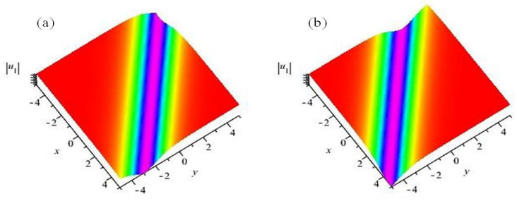
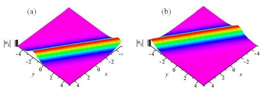
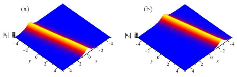
A comprehensive study on the (2+1)-dimensional hyperbolic nonlinear Schrödinger (2D-HNLS) equation describing the propagation of electromagnetic fields in self-focusing and normally dispersive planar wave guides in optics is conducted in the current paper. To this end, after reducing the 2D-HNLS equation to a one-dimensional nonlinear ordinary differential (1D-NLOD) equation in the real regime using a traveling wave transformation, its optical solitons are formally obtained through a group of well-established methods such as the exponential and Kudryashov methods. Some graphical representations regarding optical solitons that are categorized as bright and dark solitons are considered to clarify the dynamics of the obtained solutions. It is noted that some of optical solitons retrieved in the current study are new and have been not retrieved previously.
Citation: Dumitru Baleanu, Kamyar Hosseini, Soheil Salahshour, Khadijeh Sadri, Mohammad Mirzazadeh, Choonkil Park, Ali Ahmadian. The (2+1)-dimensional hyperbolic nonlinear Schrödinger equation and its optical solitons[J]. AIMS Mathematics, 2021, 6(9): 9568-9581. doi: 10.3934/math.2021556

Related Papers:

Abstract

A comprehensive study on the (2+1)-dimensional hyperbolic nonlinear Schrödinger (2D-HNLS) equation describing the propagation of electromagnetic fields in self-focusing and normally dispersive planar wave guides in optics is conducted in the current paper. To this end, after reducing the 2D-HNLS equation to a one-dimensional nonlinear ordinary differential (1D-NLOD) equation in the real regime using a traveling wave transformation, its optical solitons are formally obtained through a group of well-established methods such as the exponential and Kudryashov methods. Some graphical representations regarding optical solitons that are categorized as bright and dark solitons are considered to clarify the dynamics of the obtained solutions. It is noted that some of optical solitons retrieved in the current study are new and have been not retrieved previously.

References

[1]	Y. Yıldırım, Optical solitons to Sasa-Satsuma model with modified simple equation approach, Optik, 184 (2019), 271-276.
[2]	Y. Yıldırım, Optical solitons to Sasa-Satsuma model with trial equation approach, Optik, 184 (2019), 70-74.
[3]	K. Hosseini, M. Mirzazadeh, M. Ilie, J. F. Gómez-Aguilar, Soliton solutions of the Sasa-Satsuma equation in the monomode optical fibers including the beta-derivatives, Optik, 224 (2020), 165425.
[4]	M. Mirzazadeh, M. Ekici, A. Sonmezoglu, M. Eslami, Q. Zhou. A. H. Kara, et al., Optical solitons with complex Ginzburg-Landau equation, Nonlinear Dyn., 85 (2016), 1979-2016.
[5]	M. S. Osman, D. Lu, M. M. A. Khater, R. A. M. Attia, Complex wave structures for abundant solutions related to the complex Ginzburg-Landau model, Optik, 192 (2019), 162927.
[6]	K. Hosseini, M. Mirzazadeh, M. S. Osman, M. Al Qurashi, D. Baleanu, Solitons and Jacobi elliptic function solutions to the complex Ginzburg-Landau equation, Front. Phys., 8 (2020), 225.
[7]	A. Biswas, H. Rezazadeh, M. Mirzazadeh, M. Eslami, M. Ekici, Q. Zhou, et al., Optical soliton perturbation with Fokas-Lenells equation using three exotic and efficient integration schemes, Optik, 165 (2018), 288-294.
[8]	N. A. Kudryashov, First integrals and general solution of the Fokas-Lenells equation, Optik, 195 (2019), 163135.
[9]	K. Hosseini, M. Mirzazadeh, J. Vahidi, R. Asghari, Optical wave structures to the Fokas-Lenells equation, Optik, 207 (2020), 164450.
[10]	A. Biswas, R. T. Alqahtani, Chirp-free bright optical solitons for perturbed Gerdjikov-Ivanov equation by semi-inverse variational principle, Optik, 147 (2017), 72-76.
[11]	E. Yaşar, Y. Yıldırım, E. Yaşar, New optical solitons of space-time conformable fractional perturbed Gerdjikov-Ivanov equation by sine-Gordon equation method, Results Phys., 9 (2018), 1666-1672.
[12]	K. Hosseini, M. Mirzazadeh, M. Ilie, S. Radmehr, Dynamics of optical solitons in the perturbed Gerdjikov-Ivanov equation, Optik, 206 (2020), 164350.
[13]	A. Biswas, S. Arshed, Optical solitons in presence of higher order dispersions and absence of self-phase modulation, Optik, 174 (2018), 452-459.
[14]	A. I. Aliyu, M. Inc, A. Yusuf, D. Baleanu, M. Bayram, Dark-bright optical soliton and conserved vectors to the Biswas-Arshed equation with third-order dispersions in the absence of self-phase modulation, Front. Phys., 7 (2019), 28.
[15]	K. Hosseini, M. Mirzazadeh, M. Ilie, J. F. Gómez-Aguilar, Biswas-Arshed equation with the beta time derivative: Optical solitons and other solutions, Optik, 217 (2020), 164801.
[16]	N. A. Kudryashov, A generalized model for description of propagation pulses in optical fiber, Optik, 189 (2019), 42-52.
[17]	A. Biswas, M. Ekici, A. Sonmezoglu, A. S. Alshomrani, M. R. Belic, Optical solitons with Kudryashov's equation by extended trial function, Optik, 202 (2020), 163290.
[18]	E. M. E. Zayed, R. M. A. Shohib, A. Biswas, M. Ekici, L. Moraruf, A. K. Alzahrani, et al., Optical solitons with differential group delay for Kudryashov's model by the auxiliary equation mapping method, Chinese J. Phys., 67 (2020), 631-645.
[19]	B. K. Tan, R. S. Wu, Nonlinear Rossby waves and their interactions (I) - Collision of envelope solitary Rossby waves, Sci. China, Ser. B, 36 (1993), 1367.
[20]	S. P. Gorza, M. Haelterman, Ultrafast transverse undulation of self-trapped laser beams, Opt. Express, 16 (2008), 16935.
[21]	S. P. Gorza, P. Kockaert, P. Emplit, M. Haelterman, Oscillatory neck instability of spatial bright solitons in hyperbolic systems, Phys. Rev. Lett., 102 (2009), 134101.
[22]	G. Ai-Lin, L. Ji, Exact solutions of (2+1)-dimensional HNLS equation, Commun. Theor. Phys., 54 (2010), 401-406.
[23]	A. I. Aliyu, M. Inc, A. Yusuf, D. Baleanu, Optical solitary waves and conservation laws to the (2+1)-dimensional hyperbolic nonlinear Schrödinger equation, Mod. Phys. Lett. B, 32 (2018), 1850373.
[24]	W. O. Apeanti, A. R. Seadawy, D. Lu, Complex optical solutions and modulation instability of hyperbolic Schrödinger dynamical equation, Results Phys., 12 (2019), 2091-2097.
[25]	H. Durur, E. Ilhan, H. Bulut, Novel complex wave solutions of the (2+1)-dimensional hyperbolic nonlinear Schrödinger equation, Fractal Fract., 4 (2020), 41.
[26]	E. Tala-Tebue, C. Tetchoka-Manemo, H. Rezazadeh, A. Bekir, Y. M. Chu, Optical solutions of the (2+1)-dimensional hyperbolic nonlinear Schrödinger equation using two different methods, Results Phys., 19 (2020), 103514.
[27]	H. Ur Rehman, M. A. Imran, N. Ullah, A. Akgül, Exact solutions of (2+1)-dimensional Schrödinger's hyperbolic equation using different techniques, Numer. Meth. Part. Differ. Equ., 2020, doi: 10.1002/num.22644. doi: 10.1002/num.22644
[28]	J. H. He, X. H. Wu, Exp-function method for nonlinear wave equations, Chaos Soliton. Fract., 30 (2006), 700-708.
[29]	A. T. Ali, E. R. Hassan, General exp_a function method for nonlinear evolution equations, Appl. Math. Comput., 217 (2010), 451-459.
[30]	K. Hosseini, M. Mirzazadeh, F. Rabiei, H. M. Baskonus, G. Yel, Dark optical solitons to the Biswas-Arshed equation with high order dispersions and absence of self-phase modulation, Optik, 209 (2020), 164576.
[31]	K. Hosseini, R. Ansari, A. Zabihi, A. Shafaroody, M. Mirzazadeh, Optical solitons and modulation instability of the resonant nonlinear Schrӧdinger equations in (3+1)-dimensions, Optik, 209 (2020), 164584.
[32]	K. Hosseini, M. S. Osman, M. Mirzazadeh, F. Rabiei, Investigation of different wave structures to the generalized third-order nonlinear Scrödinger equation, Optik, 206 (2020), 164259.
[33]	K. Hosseini, R. Ansari, F. Samadani, A. Zabihi, A. Shafaroody, M. Mirzazadeh, High-order dispersive cubic-quintic Schrödinger equation and its exact solutions, Acta Phys. Pol. A, 136 (2019), 203-207.
[34]	K. Hosseini, M. Mirzazadeh, Q. Zhou, Y. Liu, M. Moradi, Analytic study on chirped optical solitons in nonlinear metamaterials with higher order effects, Laser Phys., 29 (2019), 095402.
[35]	A. Zafar, H. Rezazadeh, K. K. Ali, On finite series solutions of conformable time-fractional Cahn-Allen equation, Nonlinear Eng., 9 (2020), 194-200.
[36]	N. A. Kudryashov, Method for finding highly dispersive optical solitons of nonlinear differential equation, Optik, 206 (2020), 163550.
[37]	N. A. Kudryashov, Highly dispersive solitary wave solutions of perturbed nonlinear Schrödinger equations, Appl. Math. Comput., 371 (2020), 124972.
[38]	N. A. Kudryashov, Highly dispersive optical solitons of the generalized nonlinear eighth-order Schrödinger equation, Optik, 206 (2020), 164335.
[39]	K. Hosseini, M. Matinfar, M. Mirzazadeh, A (3+1)-dimensional resonant nonlinear Schrödinger equation and its Jacobi elliptic and exponential function solutions, Optik, 207 (2020), 164458.
[40]	K. Hosseini, K. Sadri, M. Mirzazadeh, S. Salahshour, An integrable (2+1)-dimensional nonlinear Schrödinger system and its optical soliton solutions, Optik, 229 (2021), 166247.
[41]	H. C. Ma, Z. P. Zhang, A. P. Deng, A new periodic solution to Jacobi elliptic functions of MKdV equation and BBM equation, Acta Math. Appl. Sin., 28 (2012), 409-415.
[42]	K. Hosseini, M. Mirzazadeh, Soliton and other solutions to the (1+2)-dimensional chiral nonlinear Schrödinger equation, Commun. Theor. Phys., 72 (2020), 125008.
[43]	H. Rezazadeh, S. M. Mirhosseini-Alizamini, M. Eslami, M. Rezazadeh, M. Mirzazadeh, S. Abbagari, New optical solitons of nonlinear conformable fractional Schrödinger-Hirota equation, Optik, 172 (2018), 545-553.
[44]	H. M. Srivastava, D. Baleanu, J. A. T. Machado, M. S. Osman, H. Rezazadeh, S. Arshed, et al., Traveling wave solutions to nonlinear directional couplers by modified Kudryashov method, Phys. Scr., 95 (2020), 075217.
[45]	H. B. Han, H. J. Li, C. Q. Dai, Wick-type stochastic multi-soliton and soliton molecule solutions in the framework of nonlinear Schrödinger equation, Appl. Math. Lett., 120 (2021), 107302.
[46]	P. Li, R. Li, C. Dai, Existence, symmetry breaking bifurcation and stability of two-dimensional optical solitons supported by fractional diffraction, Opt. Express, 29 (2021), 3193-3210.
[47]	C. Q. Dai, Y. Y. Wang, Coupled spatial periodic waves and solitons in the photovoltaic photorefractive crystals, Nonlinear Dyn., 102 (2020), 1733-1741.
[48]	C. Q. Dai, Y. Y. Wang, J. F. Zhang, Managements of scalar and vector rogue waves in a partially nonlocal nonlinear medium with linear and harmonic potentials, Nonlinear Dyn., 102 (2020), 379-391.
[49]	B. H. Wang, Y. Y. Wang, C. Q. Dai, Y. X. Chen, Dynamical characteristic of analytical fractional solitons for the space-time fractional Fokas-Lenells equation, Alex. Eng. J., 59 (2020), 4699-4707.
[50]	S. Boulaaras, A. Choucha, B. Cherif, A. Alharbi, M. Abdalla, Blow up of solutions for a system of two singular nonlocal viscoelastic equations with damping, general source terms and a wide class of relaxation functions, AIMS Mathematics, 6 (2021), 4664-4676.
[51]	A. Choucha, S. Boulaaras, D. Ouchenane, M. Abdalla, I. Mekawy, A. Benbella, Existence and uniqueness for Moore-Gibson-Thompson equation with, source terms, viscoelastic memory and integral condition, AIMS Mathematics, 6 (2021), 7585-7624.

Reader Comments

Your name:*

Email:*
© 2021 the Author(s), licensee AIMS Press. This is an open access article distributed under the terms of the Creative Commons Attribution License (http://creativecommons.org/licenses/by/4.0)