Characterization and engineering properties of AMU Morasko soft clay

Robert Radaszewski; Jędrzej Wierzbicki; Robert Radaszewski; Jędrzej Wierzbicki

doi:10.3934/geosci.2019.2.235

AIMS Geosciences

2019, Volume 5, Issue 2: 235-264. doi: 10.3934/geosci.2019.2.235

Previous Article Next Article

Research article Special Issues

Characterization and engineering properties of AMU Morasko soft clay

Robert Radaszewski ,
Jędrzej Wierzbicki ^,

Institute of Geology, Adam Mickiewicz University, Poznan, Poland

Received: 12 February 2019 Accepted: 15 May 2019 Published: 27 May 2019

AMU Morasko soft clay is the normally consolidated, postglacial clayey silty sand to sandy clay, deposited during the last glaciation (Weichselian) within the marginal zone of end moraine of Posnanian Phase. These soils are characterized by low plasticity, high porosity and are fully saturated, therefore, from a geotechnical point of view they can be defined as soft clays. The over 10 meter thick complex of clayey glacial sediments is covered with fine and medium sands with single grains of gravel of the so-called first sandur level from the youngest glaciation. This kind of sediments are very common in the area of north-western Poland and, due to high compressibility, become a problematic subsoil for the shallow foundations. The high porosity and saturation also causes significant problems in obtaining high quality samples for laboratory tests. This means that in situ tests are very often the only possible and economically justifiable test methods. Extended investigations carried out on these clays, which provide reliable correlations between in situ and laboratory test results, will be very useful.
For the purpose of this research paper, a wide variety of in situ (CPTU, DMT, FVT) and laboratory (physical properties, direct shear, oedometer) tests have been carried out on the material found at the depth of up to 16 m, in the area of 8 ha, within the campus of Adam Mickiewicz University (AMU) in Poznań, Poland. Preliminary investigations (performed four years ago) showed high uniformity of the test site. The current laboratory tests were carried out on both high quality natural samples and reconstructed samples. The rate effect on the results of some of the tests was also investigated. The obtained results allowed to present a wide geological and engineering characterization of these interesting glacial deposits.

Keywords:

Citation: Robert Radaszewski, Jędrzej Wierzbicki. Characterization and engineering properties of AMU Morasko soft clay[J]. AIMS Geosciences, 2019, 5(2): 235-264. doi: 10.3934/geosci.2019.2.235

Related Papers:

[1]	Miguel Vivas-Cortez, Muhammad Aamir Ali, Artion Kashuri, Hüseyin Budak . Generalizations of fractional Hermite-Hadamard-Mercer like inequalities for convex functions. AIMS Mathematics, 2021, 6(9): 9397-9421. doi: 10.3934/math.2021546
[2]	Saad Ihsan Butt, Artion Kashuri, Muhammad Umar, Adnan Aslam, Wei Gao . Hermite-Jensen-Mercer type inequalities via Ψ-Riemann-Liouville k-fractional integrals. AIMS Mathematics, 2020, 5(5): 5193-5220. doi: 10.3934/math.2020334
[3]	Miguel Vivas-Cortez, Muhammad Uzair Awan, Muhammad Zakria Javed, Artion Kashuri, Muhammad Aslam Noor, Khalida Inayat Noor . Some new generalized $\kappa$ –fractional Hermite–Hadamard–Mercer type integral inequalities and their applications. AIMS Mathematics, 2022, 7(2): 3203-3220. doi: 10.3934/math.2022177
[4]	Jia-Bao Liu, Saad Ihsan Butt, Jamshed Nasir, Adnan Aslam, Asfand Fahad, Jarunee Soontharanon . Jensen-Mercer variant of Hermite-Hadamard type inequalities via Atangana-Baleanu fractional operator. AIMS Mathematics, 2022, 7(2): 2123-2141. doi: 10.3934/math.2022121
[5]	Yanping Yang, Muhammad Shoaib Saleem, Waqas Nazeer, Ahsan Fareed Shah . New Hermite-Hadamard inequalities in fuzzy-interval fractional calculus via exponentially convex fuzzy interval-valued function. AIMS Mathematics, 2021, 6(11): 12260-12278. doi: 10.3934/math.2021710
[6]	Yamin Sayyari, Mana Donganont, Mehdi Dehghanian, Morteza Afshar Jahanshahi . Strongly convex functions and extensions of related inequalities with applications to entropy. AIMS Mathematics, 2024, 9(5): 10997-11006. doi: 10.3934/math.2024538
[7]	Jamshed Nasir, Saber Mansour, Shahid Qaisar, Hassen Aydi . Some variants on Mercer's Hermite-Hadamard like inclusions of interval-valued functions for strong Kernel. AIMS Mathematics, 2023, 8(5): 10001-10020. doi: 10.3934/math.2023506
[8]	Tahir Ullah Khan, Muhammad Adil Khan . Hermite-Hadamard inequality for new generalized conformable fractional operators. AIMS Mathematics, 2021, 6(1): 23-38. doi: 10.3934/math.2021002
[9]	Shahid Mubeen, Rana Safdar Ali, Iqra Nayab, Gauhar Rahman, Kottakkaran Sooppy Nisar, Dumitru Baleanu . Some generalized fractional integral inequalities with nonsingular function as a kernel. AIMS Mathematics, 2021, 6(4): 3352-3377. doi: 10.3934/math.2021201
[10]	Paul Bosch, Héctor J. Carmenate, José M. Rodríguez, José M. Sigarreta . Generalized inequalities involving fractional operators of the Riemann-Liouville type. AIMS Mathematics, 2022, 7(1): 1470-1485. doi: 10.3934/math.2022087

Abstract

1. Introduction

For a convex function $\sigma:\mathrm{I}\subseteq \bf{R}\to \bf{R}$ on $\mathrm{I}$ with $\nu_{1}, \nu_{2}\in \mathrm{I}$ and $\nu_{1} < \nu_{2}$ , the Hermite-Hadamard inequality is defined by ^[1]:

$\begin{equation} \sigma\left(\frac{\nu_{1}+\nu_{2}}{2}\right) \leq \frac{1}{\nu_{2}-\nu_{1}}\int_{\nu_{1}}^{\nu_{2}}\sigma(\eta)d\eta \leq \frac{\sigma(\nu_{1})+\sigma(\nu_{2})}{2}. \end{equation}$

(1.1)

The Hermite-Hadamard integral inequality (1.1) is one of the most famous and commonly used inequalities. The recently published papers ^[2,3,4] are focused on extending and generalizing the convexity and Hermite-Hadamard inequality.

The situation of the fractional calculus (integrals and derivatives) has won vast popularity and significance throughout the previous five decades or so, due generally to its demonstrated applications in numerous seemingly numerous and great fields of science and engineering ^[5,6,7].

Now, we recall the definitions of Riemann-Liouville fractional integrals.

Definition 1.1 (^[5,6,7]). Let $\sigma\in L_{1}[\nu_{1}, \nu_{2}].$ The Riemann-Liouville integrals $J_{\nu_{1}+}^{\vartheta }\sigma$ and $J_{\nu_{2}-}^{\vartheta }\sigma$ of order $\vartheta > 0$ with $\nu_{1}\geq 0$ are defined by

$\begin{equation} J_{\nu_{1}+}^{\vartheta }\sigma(x) = \frac{1}{\Gamma (\vartheta )}\int_{\nu_{1}}^{x}(x-\eta)^{\vartheta -1}\sigma(\eta)d\eta,\; \ \ \ \nu_{1} < x \end{equation}$

(1.2)

and

$\begin{equation} J_{\nu_{2}-}^{\vartheta }\sigma(x) = \frac{1}{\Gamma (\vartheta )}\int_{x}^{\nu_{2}}(\eta-x)^{\vartheta -1}\sigma(\eta)d\eta,\; \ \ x < \nu_{2}, \end{equation}$

(1.3)

respectively. Here $\Gamma (\vartheta)$ is the well-known Gamma function and $J_{\nu_{1}+}^{0}\sigma(x) = J_{\nu_{2}-}^{0}\sigma(x) = \sigma(x).$

With a huge application of fractional integration and Hermite-Hadamard inequality, many researchers in the field of fractional calculus extended their research to the Hermite-Hadamard inequality, including fractional integration rather than ordinary integration; for example see ^{[8,9,10,11,12,13,14,15,16,17,18,19,20,21]}.

In this paper, we consider the integral inequality of Hermite-Hadamard-Mercer type that relies on the Hermite-Hadamard and Jensen-Mercer inequalities. For this purpose, we recall the Jensen-Mercer inequality: Let $0 < x_{1}\leq x_{2}\leq \cdots\leq x_{n}$ and $\mu = (\mu _{1}, \mu_{2}, \ldots, \mu _{n})$ nonnegative weights such that $\sum_{i = 1}^{n}\mu_{i} = 1$ . Then, the Jensen inequality ^[22,23] is as follows, for a convex function $\sigma$ on the interval $[\nu_{1}, \nu_{2}]$ , we have

$\begin{equation} \sigma\Bigg(\sum\limits_{i = 1}^{n}\mu _{i}x_{i}\Bigg)\leq \sum\limits_{i = 1}^{n}\mu _{i}\sigma(x_{i}), \end{equation}$

(1.4)

where for all $x_{i}\in \lbrack \nu_{1}, \nu_{2}]$ and $\mu_{i}\in \lbrack 0, 1]$ , $(i = \overline{1, n})$ .

Theorem 1.1 (^[2,23]). If $\sigma$ is convex function on $[\nu_{1}, \nu_{2}]$ , then

$\begin{equation} \sigma\left(\nu_{1}+\nu_{2}-\sum\limits^{n}_{i = 1}\mu_{i}x_{i}\right)\leq \sigma(\nu_{1})+\sigma(\nu_{2})-\sum\limits^{n}_{i = 1}\mu_{i}\sigma(x_{i}), \end{equation}$

(1.5)

for each $x_{i}\in[\nu_{1}, \nu_{2}]$ and $\mu_{i}\in[0, 1]$ , $(i = \overline{1, n})$ with $\sum^{n}_{i = 1}\mu_{i} = 1$ . For some results related with Jensen-Mercer inequality, see ^[24,25,26].

In view of above indices, we establish new integral inequalities of Hermite-Hadamard-Mercer type for convex functions via the Riemann-Liouville fractional integrals in the current project. Particularly, we see that our results can cover the previous researches.

2. Main results

Theorem 2.1. For a convex function $\sigma:[\nu_{1}, \nu_{2}]\subseteq \bf{R} \to\bf{R}$ with $x, y\in[\nu_{1}, \nu_{2}]$ , we have:

$\begin{multline} \sigma\left(\nu_{1}+\nu_{2}-\frac{x+y}{2}\right)\leq \frac{2^{\vartheta -1} \Gamma\left(\vartheta +1\right)}{\left( y-x\right)^{\vartheta}} \Biggl[ J_{\left(\nu_{1}+\nu_{2}-y\right)+}^{\vartheta}\sigma\left(\nu_{1}+\nu_{2}-\frac{x+y}{2}\right) \\ +\; J_{\left(\nu_{1}+\nu_{2}-x\right)-}^{\vartheta}\sigma\left(\nu_{1}+\nu_{2}-\frac{x+y}{2}\right)\Biggr] \leq \sigma\left(\nu_{1}\right)+\sigma\left(\nu_{2}\right)-\frac{\sigma\left(x\right)+\sigma\left(y\right)}{2}. \end{multline}$

(2.1)

Proof. By using the convexity of $\sigma$ , we have

$\begin{equation} \sigma\left( \nu_{1}+\nu_{2}-\frac{u+v}{2}\right) \leq \frac{1}{2}\left[ \sigma\left( \nu_{1}+\nu_{2}-u\right) +\sigma\left( \nu_{1}+\nu_{2}-v\right) \right], \end{equation}$

(2.2)

and above with $u = \frac{1-\eta}{2}x+\frac{1+\eta}{2}y$ , $v = \frac{1+\eta}{2}x+\frac{1-\eta}{2}y$ , where $x, y\in[\nu_{1}, \nu_{2}]$ and $\eta\in [0, 1]$ , leads to

$\begin{multline} \sigma\left( \nu_{1}+\nu_{2}-\frac{x+y}{2}\right)\leq\frac{1}{2} \Biggl[\sigma\left(\nu_{1}+\nu_{2}-\left(\frac{1-\eta}{2}x+\frac{1+\eta}{2}y\right)\right) \\ +\sigma\left(\nu_{1}+\nu_{2}-\left(\frac{1+\eta}{2}x+\frac{1-\eta}{2}y\right)\right)\Biggr]. \end{multline}$

(2.3)

Multiplying both sides of (2.3) by $\eta^{\vartheta -1}$ and then integrating with respect to $\eta$ over $[0, 1]$ , we get

$\begin{align*} \frac{1}{\vartheta }\sigma\left( \nu_{1}+\nu_{2}-\frac{x+y}{2}\right) &\leq \frac{1}{2}\left[\int_{0}^{1}\eta^{\vartheta-1} \sigma\left(\nu_{1}+\nu_{2}-\left(\frac{1-\eta}{2}x+\frac{1+\eta}{2}y\right)\right)d\eta\right. \\ &+\left. \int_{0}^{1}\eta^{\vartheta -1}\sigma\left( \nu_{1}+\nu_{2}-\left( \frac{1+\eta}{2}x+\frac{1-\eta}{2}y\right)\right)d\eta\right] \\ & = \frac{1}{2}\left[ \frac{2^{\vartheta }}{\left( y-x\right) ^{\vartheta }}\int_{\nu_{1}+\nu_{2}-y}^{\nu_{1}+\nu_{2}-\frac{x+y}{2}} \left( \left( \nu_{1}+\nu_{2}-\frac{x+y}{2}\right)-w\right) ^{\vartheta -1}\sigma\left( w\right) dw\right. \\ &\left. +\frac{2^{\vartheta}}{\left(y-x\right)^{\vartheta}}\int_{\nu_{1}+\nu_{2}-\frac{x+y}{2}}^{\nu_{1}+\nu_{2}-x} \left( w-\left( \nu_{1}+\nu_{2}-\frac{x+y}{2}\right) \right) ^{\vartheta-1}\sigma\left( w\right) dw\right] \\ & = \frac{2^{\vartheta-1}\Gamma \left(\vartheta\right)}{\left(y-x\right)^{\vartheta}} \left[J_{\left(\nu_{1}+\nu_{2}-y\right)+}^{\vartheta}\sigma\left(\nu_{1}+\nu_{2}-\frac{x+y}{2}\right) +\; J_{\left(\nu_{1}+\nu_{2}-x\right)-}^{\vartheta}\sigma\left( \nu_{1}+\nu_{2}-\frac{x+y}{2}\right) \right], \end{align*}$

and thus the proof of first inequality in (2.1) is completed.

On the other hand, we have by using the Jensen-Mercer inequality:

$\begin{eqnarray} \sigma\left( \nu_{1}+\nu_{2}-\left( \frac{1-\eta}{2}x+\frac{1+\eta}{2}y\right) \right) &\leq &\sigma\left( \nu_{1}\right) +\sigma\left( \nu_{2}\right) -\left( \frac{1-\eta}{2}\sigma\left( x\right) +\frac{1+\eta}{2}\sigma\left( y\right) \right) \end{eqnarray}$

(2.4)

$\begin{eqnarray} \sigma\left( \nu_{1}+\nu_{2}-\left( \frac{1+\eta}{2}x+\frac{1-\eta}{2}y\right) \right) &\leq &\sigma\left( \nu_{1}\right) +\sigma\left( \nu_{2}\right) -\left( \frac{1+\eta}{2}\sigma\left( x\right) +\frac{1-\eta}{2}\sigma\left( y\right) \right). \end{eqnarray}$

(2.5)

Adding inequalities (2.4) and (2.5) to get

$\begin{multline} \sigma\left( \nu_{1}+\nu_{2}-\left( \frac{1-\eta}{2}x+\frac{1+\eta}{2}y\right) \right) +\sigma\left(\nu_{1}+\nu_{2}-\left( \frac{1+\eta}{2}x+\frac{1-\eta}{2}y\right) \right) \\ \leq 2\left[\sigma\left(\nu_{1}\right)+\sigma\left(\nu_{2}\right)\right]-\left[\sigma\left(x\right)+\sigma\left(y\right)\right]. \end{multline}$

(2.6)

Multiplying both sides of (2.6) by $\eta^{\vartheta -1}$ and then integrating with respect to $\eta$ over $[0, 1]$ to obtain

$\begin{multline*} \int_{0}^{1}\eta^{\vartheta -1}\sigma\left( \nu_{1}+\nu_{2}-\left( \frac{1-\eta}{2}x+\frac{1+\eta}{2}y\right) \right)d\eta +\int_{0}^{1}\eta^{\vartheta-1}\sigma\left(\nu_{1}+\nu_{2}-\left(\frac{1+\eta}{2}x+\frac{1-\eta}{2}y\right)\right)d\eta \\ \leq \frac{2}{\vartheta}\left[\sigma\left(\nu_{1}\right)+\sigma\left(\nu_{2}\right)\right] -\frac{1}{\vartheta }\left[ \sigma\left( x\right) +\sigma\left( y\right) \right]. \end{multline*}$

By making use of change of variables and then multiplying by $\frac{\vartheta }{2}$ , we get the second inequality in (2.1).

Remark 2.1. If we choose $\vartheta = 1$ , $x = \nu_{1}$ and $y = \nu_{2}$ in Theorem 2.1, then the inequality (2.1) reduces to (1.1).

Corollary 2.1. Theorem 2.1 with

● $\vartheta = 1$ becomes [24, Theorem 2.1].

● $x = \nu_{1}$ and $y = \nu_{2}$ becomes:

$\begin{align*} \sigma\left(\frac{\nu_{1}+\nu_{2}}{2}\right)\leq\frac{2^{\vartheta-1}\Gamma\left(\vartheta+1\right)}{\left(\nu_{2}-\nu_{1}\right)^{\vartheta}} \left[J_{\nu_{1}+}^{\vartheta }\sigma\left(\frac{\nu_{1}+\nu_{2}}{2}\right)+\; J_{\nu_{2}-}^{\vartheta }\sigma\left(\frac{\nu_{1}+\nu_{2}}{2}\right)\right] \leq \frac{\sigma\left(\nu_{1}\right)+\sigma\left(\nu_{2}\right) }{2}, \end{align*}$

which is obtained by Mohammed and Brevik in ^[10].

The following Lemma linked with the left inequality of (2.1) is useful to obtain our next results.

Lemma 2.1. Let $\sigma:[\nu_{1}, \nu_{2}]\subseteq\bf{R} \to\bf{R}$ be a differentiable function on $(\nu_{1}, \nu_{2})$ and $\sigma'\in L[\nu_{1}, \nu_{2}]$ with $\nu_{1}\leq \nu_{2}$ and $x, y\in[\nu_{1}, \nu_{2}]$ . Then, we have:

$\begin{multline} \frac{2^{\vartheta -1}\Gamma \left( \vartheta +1\right) }{\left( y-x\right)^{\vartheta}} \left[ J_{\left( \nu_{1}+\nu_{2}-y\right) +}^{\vartheta }\sigma\left(\nu_{1}+\nu_{2}-\frac{x+y}{2}\right) +\; J_{\left( \nu_{1}+\nu_{2}-x\right)-}^{\vartheta}\sigma\left(\nu_{1}+\nu_{2}-\frac{x+y}{2}\right)\right] \\ -\sigma\left(\nu_{1}+\nu_{2}-\frac{x+y}{2}\right) = \frac{\left(y-x\right)}{4}\int_{0}^{1}\eta^{\vartheta} \Bigl[\sigma'\left(\nu_{1}+\nu_{2}-\left(\frac{1-\eta}{2}x+\frac{1+\eta}{2}y\right)\right) \\ -\sigma'\left(\nu_{1}+\nu_{2}-\left(\frac{1+\eta}{2}x+\frac{1-\eta}{2}y\right)\right)\Bigr]d\eta. \end{multline}$

(2.7)

Proof. From right hand side of (2.7), we set

$\begin{align} \varpi_{1}-\varpi_{2}&:= \int_{0}^{1}\eta^{\vartheta}\left[\sigma'\left(\nu_{1}+\nu_{2} -\left(\frac{1-\eta}{2}x+\frac{1+\eta}{2}y\right)\right) -\sigma'\left( \nu_{1}+\nu_{2}-\left( \frac{1+\eta}{2}x+\frac{1-\eta}{2}y\right)\right)\right]d\eta \\ & = \int_{0}^{1}\eta^{\vartheta }\sigma'\left(\nu_{1}+\nu_{2}-\left(\frac{1-\eta}{2}x+\frac{1+\eta}{2}y\right)\right)d\eta \\ &-\int_{0}^{1}\eta^{\vartheta}\sigma'\left(\nu_{1}+\nu_{2}-\left(\frac{1+\eta}{2}x+\frac{1-\eta}{2}y\right)\right) d\eta. \end{align}$

(2.8)

By integrating by parts with $w = \nu_{1}+\nu_{2}-\left(\frac{1-\eta}{2}x+\frac{1+\eta}{2}y\right)$ , we can deduce:

$\begin{align*} \varpi_{1}& = -\frac{2}{\left( y-x\right) }\sigma\left(\nu_{1}+\nu_{2}-y\right)+\frac{2\vartheta }{\left(y-x\right)} \int_{0}^{1}\eta^{\vartheta -1}\sigma\left( \nu_{1}+\nu_{2}-\left( \frac{1-\eta}{2}x+\frac{1+\eta}{2}y\right) \right) d\eta \\ & = -\frac{2}{\left(y-x\right)}\sigma\left(\nu_{1}+\nu_{2}-y\right)+\frac{2^{\vartheta+1}\vartheta}{\left(y-x\right)^{\vartheta+1}} \int_{\nu_{1}+\nu_{2}-y}^{\nu_{1}+\nu_{2}-\frac{x+y}{2}}\sigma\left(\left( \nu_{1}+\nu_{2}-\frac{x+y}{2}\right)-w\right)^{\vartheta -1} \sigma\left(w\right) dw \\ & = -\frac{2}{\left(y-x\right)}\sigma\left( \nu_{1}+\nu_{2}-y\right) +\frac{2^{\vartheta+1}\Gamma\left(\vartheta+1\right)}{\left( y-x\right) ^{\vartheta +1}} J_{\left(\nu_{1}+\nu_{2}-y\right)+}^{\vartheta }\sigma\left( \nu_{1}+\nu_{2}-\frac{x+y}{2}\right). \end{align*}$

Similarly, we can deduce:

$\begin{equation*} \varpi_{2} = \frac{2}{y-x}\sigma\left(\nu_{1}+\nu_{2}-x\right) -\frac{2^{\vartheta+1}\Gamma\left(\vartheta+1\right)}{\left( y-x\right) ^{\vartheta +1}} J_{\left( \nu_{1}+\nu_{2}-x\right)-}^{\vartheta }\sigma\left(\nu_{1}+\nu_{2}-\frac{x+y}{2}\right). \end{equation*}$

By substituting $\varpi_{1}$ and $\varpi_{2}$ in (2.8) and then multiplying by $\frac{\left(y-x\right)}{4}$ , we obtain required identity (2.7).

Corollary 2.2. Lemma 2.1 with

● $\vartheta = 1$ becomes:

$\begin{multline*} \frac{1}{y-x}\int_{\nu_{1}+\nu_{2}-y}^{\nu_{1}+\nu_{2}-x}\sigma\left(w\right) dw-\sigma\left( \nu_{1}+\nu_{2}-\frac{x+y}{2}\right) = \frac{\left( y-x\right) }{4}\int_{0}^{1}\eta\left[ \sigma'\left( \nu_{1}+\nu_{2}-\left( \frac{1-\eta}{2}x+\frac{1+\eta}{2}y\right) \right) \right. \\ \left. -\sigma'\left( \nu_{1}+\nu_{2}-\left( \frac{1+\eta}{2}x+\frac{1-\eta}{2}y\right)\right) \right] d\eta. \end{multline*}$

● $\vartheta = 1$ , $x = \nu_{1}$ and $y = \nu_{2}$ becomes:

$\begin{multline*} \frac{1}{\nu_{2}-\nu_{1}}\int_{\nu_{1}}^{\nu_{2}}\sigma\left( w\right) dw-\sigma\left(\frac{\nu_{1}+\nu_{2}}{2}\right) = \frac{\left( \nu_{2}-\nu_{1}\right) }{4}\int_{0}^{1}\eta \left[ \sigma'\left(\nu_{1}+\nu_{2}-\left( \frac{1-\eta}{2}\nu_{1}+\frac{1+\eta}{2}\nu_{2}\right) \right) \right. \\ \left. -\sigma'\left( \nu_{1}+\nu_{2}-\left( \frac{1+\eta}{2}\nu_{1}+\frac{1-\eta}{2}\nu_{2}\right)\right) \right] d\eta. \end{multline*}$

● $x = \nu_{1}$ and $y = \nu_{2}$ becomes:

$\begin{multline*} \frac{2^{\vartheta -1}\Gamma \left( \vartheta +1\right) }{\left( \nu_{2}-\nu_{1}\right)^{\vartheta }} \left[ J_{\nu_{1}+}^{\vartheta }\sigma\left(\frac{\nu_{1}+\nu_{2}}{2}\right) +\; J_{\nu_{2}-}^{\vartheta }\sigma\left(\frac{\nu_{1}+\nu_{2}}{2}\right) \right]-\sigma\left(\frac{\nu_{1}+\nu_{2}}{2}\right) \\ = \frac{\left( \nu_{2}-\nu_{1}\right) }{4}\int_{0}^{1}\eta^{\vartheta } \left[\sigma'\left( \nu_{1}+\nu_{2}-\left( \frac{1-\eta}{2}\nu_{1}+\frac{1+\eta}{2}\nu_{2}\right) \right) \right. \left. -\sigma'\left( \nu_{1}+\nu_{2}-\left( \frac{1+\eta}{2}\nu_{1}+\frac{1-\eta}{2}\nu_{2}\right) \right) \right] d\eta. \end{multline*}$

Theorem 2.2. Let $\sigma:[\nu_{1}, \nu_{2}]\subseteq\bf{R}\to\bf{R}$ be a differentiable function on $(\nu_{1}, \nu_{2})$ and $|\sigma'|$ is convex on $[\nu_{1}, \nu_{2}]$ with $\nu_{1}\leq \nu_{2}$ and $x, y\in[\nu_{1}, \nu_{2}]$ . Then, we have:

$\begin{multline} \Biggl| \frac{2^{\vartheta -1}\Gamma \left( \vartheta +1\right) }{\left(y-x\right) ^{\vartheta }} \Biggl[ J_{\left( \nu_{1}+\nu_{2}-y\right) +}^{\vartheta }\sigma\left( \nu_{1}+\nu_{2}-\frac{x+y}{2}\right) +\; J_{\left( \nu_{1}+\nu_{2}-x\right) -}^{\vartheta }\sigma\left( \nu_{1}+\nu_{2}-\frac{x+y}{2}\right) \Biggr] \\ -\sigma\left( \nu_{1}+\nu_{2}-\frac{x+y}{2}\right)\Biggr| \leq \frac{\left( y-x\right) }{2\left( 1+\vartheta \right) }\left[ \left| \sigma'\left( \nu_{1}\right) \right| +\left| \sigma'\left(\nu_{2}\right) \right| -\frac{\left| \sigma'\left( x\right) \right| +\left| \sigma'\left( y\right) \right| }{2}\right]. \end{multline}$

(2.9)

Proof. By taking modulus of identity (2.7), we get

$\begin{multline*} \Biggl|\frac{2^{\vartheta-1}\Gamma\left(\vartheta+1\right)}{\left(y-x\right)^{\vartheta}} \left[J_{\left(\nu_{1}+\nu_{2}-y\right)+}^{\vartheta}\sigma\left(\nu_{1}+\nu_{2}-\frac{x+y}{2}\right) +\; J_{\left( \nu_{1}+\nu_{2}-x\right) -}^{\vartheta }\sigma\left( \nu_{1}+\nu_{2}-\frac{x+y}{2}\right) \right] \\ -\sigma\left( \nu_{1}+\nu_{2}-\frac{x+y}{2}\right) \Biggr|\leq \frac{\left( y-x\right) }{4} \left[\int_{0}^{1}\eta^{\vartheta }\left|\sigma'\left( \nu_{1}+\nu_{2}-\left( \frac{1-\eta}{2}x+\frac{1+\eta}{2}y\right) \right) \right| d\eta\right. \\ \left. +\int_{0}^{1}\eta^{\vartheta }\left| \sigma'\left( \nu_{1}+\nu_{2}-\left( \frac{1+\eta}{2}x+\frac{1-\eta}{2}y\right) \right) \right| d\eta\right]. \end{multline*}$

Then, by applying the convexity of $|\sigma'|$ and the Jensen-Mercer inequality on above inequality, we get

$\begin{align*} &\Biggl|\frac{2^{\vartheta-1}\Gamma\left(\vartheta+1\right)}{\left(y-x\right)^{\vartheta}} \left[J_{\left(\nu_{1}+\nu_{2}-y\right)+}^{\vartheta}\sigma\left(\nu_{1}+\nu_{2}-\frac{x+y}{2}\right) +\; J_{\left( \nu_{1}+\nu_{2}-x\right) -}^{\vartheta }\sigma\left( \nu_{1}+\nu_{2}-\frac{x+y}{2}\right) \right] \\ &-\sigma\left( \nu_{1}+\nu_{2}-\frac{x+y}{2}\right) \Biggr|\leq \frac{\left( y-x\right) }{4}\left[ \int_{0}^{1}\eta^{\vartheta }\left[ \left| \sigma'\left( \nu_{1}\right) \right| +\left| \sigma'\left( \nu_{2}\right) \right| -\left( \frac{1+\eta}{2}\left| \sigma^{\prime }\left( x\right) \right| +\frac{1-\eta}{2}\right) \left| \sigma'\left( y\right) \right| \right] d\eta\right. \\ &\left. +\int_{0}^{1}\eta^{\vartheta }\left[ \left| \sigma'\left(\nu_{1}\right) \right| +\left| \sigma'\left( \nu_{2}\right) \right| -\left(\frac{1-\eta}{2}\left|\sigma'\left(x\right) \right| +\frac{1+\eta}{2}\right)\left| \sigma'\left( y\right)\right| \right] d\eta\right] \\ & = \frac{\left(y-x\right)}{2\left(1+\vartheta \right)}\left[ \left|\sigma'\left( \nu_{1}\right)\right| +\left|\sigma'(\nu_{2})\right|-\frac{\left|\sigma'\left(x\right)\right|+\left|\sigma'\left(y\right)\right|}{2}\right], \end{align*}$

which completes the proof of Theorem 2.2.

Corollary 2.3. Theorem 2.2 with

● $\vartheta = 1$ becomes:

$\begin{align*} \left|\frac{1}{y-x}\int_{\nu_{1}+\nu_{2}-y}^{\nu_{1}+\nu_{2}-x}\sigma(w)dw-\sigma\left(\nu_{1}+\nu_{2}-\frac{x+y}{2}\right)\right| \leq \frac{\left(y-x\right)}{4}\left[\left| \sigma'\left(\nu_{1}\right)\right|+\left|\sigma'\left(\nu_{2}\right)\right| -\frac{\left|\sigma'\left(x\right)\right|+\left|\sigma'\left(y\right)\right|}{2}\right]. \end{align*}$

● $\vartheta = 1$ , $x = \nu_{1}$ and $y = \nu_{2}$ becomes [27, Theorem 2.2].

● $x = \nu_{1}$ and $y = \nu_{2}$ becomes:

$\begin{align*} \left\vert \frac{1}{\nu_{2}-\nu_{1}}\int_{\nu_{1}}^{\nu_{2}}\sigma\left( w\right) dw-\sigma\left(\frac{\nu_{1}+\nu_{2}}{2}\right) \right\vert \leq \frac{\left( \nu_{2}-\nu_{1}\right) }{4}\left[ \frac{\left\vert \sigma^{\prime }\left( \nu_{1}\right) \right\vert +\left\vert \sigma^{\prime }\left( \nu_{2}\right) \right\vert }{2}\right] . \end{align*}$

Theorem 2.3. Let $\sigma:[\nu_{1}, \nu_{2}]\subseteq\bf{R}\to\bf{R}$ be a differentiable function on $(\nu_{1}, \nu_{2})$ and $\left| \sigma'\right|^{q}, q > 1$ is convex on $[\nu_{1}, \nu_{2}]$ with $\nu_{1}\leq \nu_{2}$ and $x, y\in[\nu_{1}, \nu_{2}]$ . Then, we have:

$\begin{multline} \left| \frac{2^{\vartheta -1}\Gamma \left( \vartheta +1\right) }{\left( y-x\right) ^{\vartheta }}\left[ J_{\left( \nu_{1}+\nu_{2}-y\right) +}^{\vartheta }\sigma\left( \nu_{1}+\nu_{2}- \frac{x+y}{2}\right) \right. \right. \\ \left. \left. +\; J_{\left( \nu_{1}+\nu_{2}-x\right) -}^{\vartheta }\sigma\left(\nu_{1}+\nu_{2}-\frac{x+y}{2}\right) \right] -\sigma\left( \nu_{1}+\nu_{2}-\frac{x+y}{2}\right) \right| \\ \leq \frac{\left( y-x\right) }{4\sqrt[p]{\vartheta p+1}} \left[ \left( \left| \sigma'\left( \nu_{1}\right) \right|^{q}+\left| \sigma'\left(\nu_{2}\right)\right| ^{q} -\left(\frac{\left|\sigma'(x) \right|^{q}+3\left|\sigma'(y)\right|^{q}}{4}\right)\right)^{\frac{1}{q}}\right. \\ \left. +\left( \left| \sigma'\left( \nu_{1}\right) \right|^{q}+\left|\sigma'\left(\nu_{2}\right)\right|^{q} -\left(\frac{3\left|\sigma'(x)\right|^{q}+\left|\sigma'(y)\right|^{q}}{4}\right)\right)^{\frac{1}{q}}\right], \end{multline}$

(2.10)

where $\frac{1}{p}+\frac{1}{q} = 1$ .

Proof. By taking modulus of identity (2.7) and using Hölder's inequality, we get

$\begin{multline*} \left| \frac{2^{\vartheta -1}\Gamma \left( \vartheta +1\right) }{\left(y-x\right)^{\vartheta }} \left[ J_{\left( \nu_{1}+\nu_{2}-y\right)+}^{\vartheta }\sigma\left( \nu_{1}+\nu_{2}-\frac{x+y}{2}\right) \right. \right. \\ \left. \left. +\; J_{\left(\nu_{1}+\nu_{2}-x\right)-}^{\vartheta }\sigma\left(\nu_{1}+\nu_{2}-\frac{x+y}{2}\right) \right] -\sigma\left( \nu_{1}+\nu_{2}-\frac{x+y}{2}\right) \right| \\ \leq \frac{\left( y-x\right) }{4}\left( \int_{0}^{1}\eta^{\vartheta p}\right)^{\frac{1}{p}} \left\{\left(\int_{0}^{1} \left|\sigma'\left(\nu_{1}+\nu_{2}-\left(\frac{1-\eta}{2}x+\frac{1+\eta}{2}y\right)\right)\right|^{q}d\eta\right) ^{\frac{1}{q}}\right. \\ \left. +\left(\int_{0}^{1} \left|\sigma'\left(\nu_{1}+\nu_{2}-\left(\frac{1+\eta}{2}x+\frac{1-\eta}{2}y\right)\right)\right|^{q}d\eta\right) ^{\frac{1}{q}}\right\}. \end{multline*}$

Then, by applying the Jensen-Mercer inequality with the convexity of $\left|\sigma'\right|^{q}$ , we can deduce

$\begin{align*} &\left| \frac{2^{\vartheta -1}\Gamma \left( \vartheta +1\right) }{\left(y-x\right) ^{\vartheta }} \left[J_{\left(\nu_{1}+\nu_{2}-y\right)+}^{\vartheta }\sigma\left( \nu_{1}+\nu_{2}-\frac{x+y}{2}\right) \right. \right. \\ &\left. \left. +\; J_{\left( \nu_{1}+\nu_{2}-x\right) -}^{\vartheta }\sigma\left( \nu_{1}+\nu_{2}-\frac{x+y}{2}\right) \right] -\sigma\left( \nu_{1}+\nu_{2}-\frac{x+y}{2}\right) \right| \\ &\leq \frac{\left( y-x\right) }{4}\left( \int_{0}^{1}\eta^{\vartheta p}\right)^{\frac{1}{p}} \left\{ \left( \int_{0}^{1}\left| \sigma'\left( \nu_{1}\right)\right| ^{q}+\left| \sigma'\left( \nu_{2}\right) \right|^{q} -\left(\frac{1-\eta}{2}\left|\sigma'(x)\right|^{q}+\frac{1+\eta}{2}\left|\sigma'(y)\right|^{q}\right)\right)^{\frac{1}{q}}\right. \\ &\left. +\left( \int_{0}^{1}\left| \sigma'\left( \nu_{1}\right)\right| ^{q}+\left| \sigma'\left( \nu_{2}\right) \right|^{q} -\left(\frac{1+\eta}{2}\left| \sigma'\left( x\right)\right|^{q}+\frac{1-\eta}{2}\left| \sigma'\left( y\right) \right|^{q} \right) \right)^{\frac{1}{q}}\right\} \\ & = \frac{\left(y-x\right)}{4\sqrt[p]{\vartheta p+1}}\left[\left( \left| \sigma'\left( \nu_{1}\right) \right| ^{q} +\left|\sigma'\left( \nu_{2}\right) \right| ^{q}-\left( \frac{\left|\sigma'\left( x\right) \right|^{q} +3\left| \sigma'\left(y\right) \right|^{q} }{4}\right) \right) ^{\frac{1}{q}}\right. \\ &\left. +\left( \left| \sigma'\left( \nu_{1}\right) \right|^{q}+\left| \sigma'\left( \nu_{2}\right) \right| ^{q} -\left(\frac{3\left|\sigma'(x)\right|^{q}+\left|\sigma'(y)\right|^{q}}{4}\right)\right)^{\frac{1}{q}}\right], \end{align*}$

which completes the proof of Theorem 2.3.

Corollary 2.4. Theorem 2.3 with

● $\vartheta = 1$ becomes:

$\begin{multline*} \left|\frac{1}{y-x}\int_{\nu_{1}+\nu_{2}-y}^{\nu_{1}+\nu_{2}-x}\sigma\left(w\right)dw -\sigma\left(\nu_{1}+\nu_{2}-\frac{x+y}{2}\right)\right| \\ \leq \frac{\left( y-x\right)}{4\sqrt[p]{p+1}}\left[\left( \left| \sigma'\left( \nu_{1}\right) \right|^{q} +\left|\sigma'\left( \nu_{2}\right) \right| ^{q}-\left( \frac{\left|\sigma'\left( x\right) \right|^{q} +3\left|\sigma'\left(y\right) \right|^{q}}{4}\right)\right)^{\frac{1}{q}}\right. \\ \left. +\left(\left|\sigma'\left( \nu_{1}\right)\right|^{q}+\left| \sigma'\left( \nu_{2}\right)\right|^{q} -\left(\frac{3\left|\sigma'(x)\right|^{q}+\left|\sigma'(y)\right|^{q} }{4}\right)\right)^{\frac{1}{q}}\right]. \end{multline*}$

● $\vartheta = 1$ , $x = \nu_{1}$ and $y = \nu_{2}$ becomes:

$\begin{align*} &&\left\vert \frac{1}{\nu_{2}-\nu_{1}}\int_{\nu_{1}}^{\nu_{2}}\sigma\left( w\right) dw-\sigma\left(\frac{\nu_{1}+\nu_{2}}{2}\right) \right\vert \leq \frac{\left( \nu_{2}-\nu_{1}\right) }{2^{\frac{2}{p}}}\left(\frac{1}{p+1}\right)^{\frac{1}{p}}\left[ \left\vert \sigma^{\prime }\left( \nu_{1}\right) \right\vert +\left\vert \sigma^{\prime }\left( \nu_{2}\right) \right\vert \right] . \end{align*}$

● $x = \nu_{1}$ and $y = \nu_{2}$ becomes:

$\begin{align*} &\left\vert \frac{2^{\vartheta-1}\Gamma\left(\vartheta+1\right)}{\left(\nu_{2}-\nu_{1}\right)^{\vartheta}} \left[ J_{\nu_{1}+}^{\vartheta }\sigma\left(\frac{\nu_{1}+\nu_{2}}{2}\right) \right. \right. \left. \left. +\; J_{\nu_{2}-}^{\vartheta }\sigma\left(\frac{\nu_{1}+\nu_{2}}{2}\right) \right] -\sigma\left(\frac{\nu_{1}+\nu_{2}}{2}\right) \right\vert \\ &\leq \frac{2^{\vartheta-1-\frac{2}{q}}}{\nu_{2}-\nu_{1}}\left(\frac{1}{p+1}\right)^{\frac{1}{p}}\left[ \left\vert \sigma'\left( \nu_{1}\right) \right\vert +\left\vert \sigma'\left( \nu_{2}\right) \right\vert \right]. \end{align*}$

Theorem 2.4. Let $\sigma:[\nu_{1}, \nu_{2}]\subseteq\bf{R}\to\bf{R}$ be a differentiable function on $(\nu_{1}, \nu_{2})$ and $\left|\sigma'\right|^{q}, q\geq 1$ is convex on $[\nu_{1}, \nu_{2}]$ with $\nu_{1}\leq \nu_{2}$ and $x, y\in[\nu_{1}, \nu_{2}]$ . Then, we have:

$\begin{multline} \left| \frac{2^{\vartheta -1}\Gamma \left( \vartheta +1\right) }{\left(y-x\right) ^{\vartheta }} \left[ J_{\left( \nu_{1}+\nu_{2}-y\right) +}^{\vartheta }\sigma\left( \nu_{1}+\nu_{2}-\frac{x+y}{2}\right)\right.\right. \\ \left. \left. +\; J_{\left( \nu_{1}+\nu_{2}-x\right) -}^{\vartheta }\sigma\left( \nu_{1}+\nu_{2}-\frac{x+y}{2}\right) \right] -\sigma\left( \nu_{1}+\nu_{2}-\frac{x+y}{2}\right) \right| \\ \leq \frac{\left(y-x\right)}{4\left(\vartheta+1\right)}\left[\left(\left|\sigma'(\nu_{1})\right|^{q} +\left|\sigma'\left(\nu_{2}\right)\right|^{q}-\left( \frac{\left| \sigma'\left(x\right)\right|^{q} +\left( 2\vartheta+3\right)\left|\sigma'(y)\right|^{q}}{2\left(\vartheta+2\right) }\right)\right)^{\frac{1}{q}}\right. \\ \left. +\left( \left|\sigma'\left(\nu_{1}\right)\right|^{q}+\left| \sigma'\left( \nu_{2}\right)\right|^{q} -\left(\frac{\left(2\vartheta+3\right)\left|\sigma'(x)\right|^{q}+\left|\sigma'(y)\right|^{q}}{2\left( \vartheta+2\right) }\right) \right) ^{\frac{1}{q}}\right]. \end{multline}$

(2.11)

Proof. By taking modulus of identity (2.7) with the well-known power mean inequality, we can deduce

$\begin{multline*} \left| \frac{2^{\vartheta -1}\Gamma \left( \vartheta +1\right) }{\left(y-x\right) ^{\vartheta }} \left[ J_{\left( \nu_{1}+\nu_{2}-y\right) +}^{\vartheta }\sigma\left( \nu_{1}+\nu_{2}-\frac{x+y}{2}\right) \right. \right. \\ \left. \left. +\; J_{\left( \nu_{1}+\nu_{2}-x\right) -}^{\vartheta }\sigma\left( \nu_{1}+\nu_{2}-\frac{x+y}{2}\right) \right] -\sigma\left( \nu_{1}+\nu_{2}-\frac{x+y}{2}\right) \right| \\ \leq \frac{\left( y-x\right) }{4}\left( \int_{0}^{1}\eta^{\vartheta }\right) ^{1-\frac{1}{q}} \left\{\left(\int_{0}^{1}\eta^{\vartheta} \left|\sigma'\left(\nu_{1}+\nu_{2}-\left(\frac{1-\eta}{2}x+\frac{1+\eta}{2}y\right)\right)\right|^{q}d\eta\right)^{\frac{1}{q}}\right. \\ \left. +\left( \int_{0}^{1}\eta^{\vartheta } \left|\sigma'\left(\nu_{1}+\nu_{2}-\left(\frac{1+\eta}{2}x+\frac{1-\eta}{2}y\right)\right)\right|^{q}d\eta\right)^{\frac{1}{q}}\right\} . \end{multline*}$

By applying the Jensen-Mercer inequality with the convexity of $\left|\sigma'\right|^{q}$ , we can deduce

$\begin{align*} &\left| \frac{2^{\vartheta -1}\Gamma \left( \vartheta +1\right) }{\left(y-x\right)^{\vartheta}} \left[ J_{\left( \nu_{1}+\nu_{2}-y\right)+}^{\vartheta}\sigma\left(\nu_{1}+\nu_{2}-\frac{x+y}{2}\right) \right. \right. \\ &\left. \left. +\; J_{\left( \nu_{1}+\nu_{2}-x\right) -}^{\vartheta }\sigma\left( \nu_{1}+\nu_{2}-\frac{x+y}{2}\right)\right] -\sigma\left( \nu_{1}+\nu_{2}-\frac{x+y}{2}\right) \right| \\ &\leq \frac{\left( y-x\right)}{4}\left(\int_{0}^{1}\eta^{\vartheta }\right)^{1-\frac{1}{q}} \left\{ \left( \int_{0}^{1}\eta^{\vartheta }\left[ \left|\sigma'\left( \nu_{1}\right) \right|^{q} +\left| \sigma'\left(\nu_{2}\right) \right| ^{q}-\left( \frac{1-\eta}{2}\left| \sigma'\left(x\right)\right|^{q} +\frac{1+\eta}{2}\left| \sigma'\left( y\right)\right| ^{q}\right) \right] \right) ^{\frac{1}{q}}\right. \\ &\left. +\left( \int_{0}^{1}\eta^{\vartheta }\left[ \left| \sigma'\left(\nu_{1}\right)\right|^{q} +\left| \sigma'\left( \nu_{2}\right) \right|^{q}-\left( \frac{1+\eta}{2}\left| \sigma'\left( x\right) \right|^{q} +\frac{1-\eta}{2}\left| \sigma'\left( y\right) \right|^{q}\right) \right] \right) ^{\frac{1}{q}}\right\} \\ & = \frac{\left( y-x\right) }{4\left( \vartheta +1\right) }\left[\left(\left|\sigma'\left(\nu_{1}\right)\right|^{q} +\left|\sigma'\left( \nu_{2}\right) \right| ^{q}-\left( \frac{\left| \sigma'\left(x\right) \right|^{q} +\left(2\vartheta +3\right)\left|\sigma'(y)\right|^{q}}{2\left(\vartheta+2\right)}\right)\right)^{\frac{1}{q}}\right. \\ &\left. +\left( \left| \sigma'\left( \nu_{1}\right) \right|^{q}+\left|\sigma'\left( \nu_{2}\right)\right|^{q} -\left( \frac{\left( 2\vartheta +3\right) \left| \sigma'\left( x\right) \right|^{q} +\left|\sigma'\left( y\right)\right|^{q}}{2\left(\vartheta+2\right)}\right)\right)^{\frac{1}{q}}\right], \end{align*}$

which completes the proof of Theorem 2.4.

Corollary 5. Theorem 2.4 with

● $q = 1$ becomes Theorem 2.2.

● $\vartheta = 1$ becomes:

$\begin{multline*} \left| \frac{1}{y-x}\int_{\nu_{1}+\nu_{2}-y}^{\nu_{1}+\nu_{2}-x}\sigma\left(w\right) dw -\sigma\left( \nu_{1}+\nu_{2}-\frac{x+y}{2}\right) \right| \\ \leq \frac{\left( y-x\right) }{8}\left[ \left( \left|\sigma'\left( \nu_{1}\right)\right|^{q} +\left| \sigma'\left( \nu_{2}\right)\right|^{q}-\left( \frac{\left| \sigma'\left( x\right)\right|^{q} +5\left|\sigma'\left(y\right)\right|^{q}}{6}\right)\right)^{\frac{1}{q}}\right. \\ \left. +\left( \left| \sigma'\left( \nu_{1}\right) \right|^{q}+\left|\sigma'\left(\nu_{2}\right)\right|^{q} -\left(\frac{5\left|\sigma'(x)\right|^{q}+\left|\sigma'(y)\right|^{q}}{6}\right)\right)^{\frac{1}{q}}\right]. \end{multline*}$

● $\vartheta = 1$ , $x = \nu_{1}$ and $y = \nu_{2}$ becomes:

$\begin{multline*} \left| \frac{1}{\nu_{2}-\nu_{1}}\int_{\nu_{1}}^{\nu_{2}}\sigma\left( w\right) dw -\sigma\left(\frac{\nu_{1}+\nu_{2}}{2}\right)\right| \\ \leq \frac{\left(y-x\right)}{8}\left[\left(\frac{5\left|\sigma'\left(\nu_{1}\right)\right|^{q} +\left| \sigma'\left( \nu_{2}\right)\right| ^{q}}{6}\right)^{\frac{1}{q}} +\left(\frac{\left|\sigma'(\nu_{1})\right|^{q}+5\left| \sigma'(\nu_{2})\right|^{q}}{6}\right)^{\frac{1}{q}}\right]. \end{multline*}$

● $x = \nu_{1}$ and $y = \nu_{2}$ becomes:

$\begin{multline*} \left| \frac{2^{\vartheta-1}\Gamma\left(\vartheta+1\right)}{\left(\nu_{2}-\nu_{1}\right)^{\vartheta}} \left[J_{\nu_{1} +}^{\vartheta}\sigma\left(\frac{\nu_{1}+\nu_{2}}{2}\right)+\; J_{\nu_{2} -}^{\vartheta }\sigma\left( \frac{\nu_{1}+\nu_{2}}{2}\right)\right] -\sigma\left( \frac{\nu_{1}+\nu_{2}}{2}\right)\right| \\ \leq \frac{\left(\nu_{2}-\nu_{1}\right)}{4\left(\vartheta+1\right)} \left[\left(\frac{\left(2\vartheta+3\right)\left|\sigma'(\nu_{1})\right|^{q}+\left|\sigma'(\nu_{2})\right|^{q}}{2\left(\vartheta+2\right)}\right)^{\frac{1}{q}} +\left(\frac{\left|\sigma'(\nu_{1})\right|^{q}+\left(2\vartheta+3\right)\left|\sigma'(\nu_{2})\right|^{q}}{2\left(\vartheta+2\right)}\right) ^{\frac{1}{q}}\right]. \end{multline*}$

3. Applications to special means

Here, we consider the following special means:

● The arithmetic mean:

$\mathcal{A}(\nu_{1},\nu_{2}) = \frac{\nu_{1}+\nu_{2}}{2}, \quad \nu_{1}, \nu_{2}\geq 0.$

● The harmonic mean:

$\mathcal{H}(\nu_{1},\nu_{2}) = \frac{2\nu_{1}\nu_{2}}{\nu_{1}+\nu_{2}}, \quad \nu_{1}, \nu_{2} > 0.$

● The logarithmic mean:

$\begin{equation*} \mathcal{L}(\nu_{1},\nu_{2}) = \begin{cases} \frac{\nu_{2}-\nu_{1}}{\ln \nu_{2}-\ln \nu_{1}}, & \text{if}\; \nu_{1}\neq \nu_{2}, \\ \nu_{1}, & \text{if}\; \nu_{1} = \nu_{2}, \end{cases} \quad \nu_{1}, \nu_{2} > 0. \end{equation*}$

● The generalized logarithmic mean:

$\begin{equation*} \mathcal{L}_{n}(\nu_{1},\nu_{2}) = \begin{cases} \left[\frac{\nu_{2}^{n+1}-\nu_{1}^{n+1}}{\left(n+1\right)(\nu_{2}-\nu_{1})}\right]^{\frac{1}{n}}, & \text{if}\; \nu_{1}\neq \nu_{2} \\ \nu_{1}, & \text{if}\; \nu_{1} = \nu_{2}, \end{cases} \quad \nu_{1},\nu_{2} > 0;\; n\in\bf{Z}\setminus \{-1,0\}. \end{equation*}$

Proposition 3.1. Let $0 < \nu_{1} < \nu_{2}$ and $n\in\bf{N}$ , $n \geq 2$ . Then, for all $x, y\in[\nu_{1}, \nu_{2}]$ , we have:

(3.1)

Proof. By applying Corollary 2.3 (first item) for the convex function $\sigma(x) = x^{n}, \, x > 0$ , one can obtain the result directly.

Proposition 3.2. Let $0 < \nu_{1} < \nu_{2}$ . Then, for all $x, y\in[\nu_{1}, \nu_{2}]$ , we have:

(3.2)

Proof. By applying Corollary 2.3 (first item) for the convex function $\sigma(x) = \frac{1}{x}, \, x > 0$ , one can obtain the result directly.

Proposition 3.3. Let $0 < \nu_{1} < \nu_{2}$ and $n\in\bf{N}$ , $n \geq 2$ . Then, we have:

$\begin{equation} \left| \mathcal{L}_{n}^{n}(\nu_{1},\nu_{2}) -\mathcal{A}^{n}(\nu_{1},\nu_{2}) \right| \leq \frac{n(\nu_{2}-\nu_{1})}{4} \left[ \mathcal{A}\left(\nu_{1}^{n-1}, \nu_{2}^{n-1}\right) \right], \end{equation}$

(3.3)

and

$\begin{equation} \left| \mathcal{L}^{-1}(\nu_{1},\nu_{2}) -\mathcal{A}^{-1}(\nu_{1},\nu_{2}) \right| \leq \frac{(\nu_{2}-\nu_{1})}{4}\mathcal{H}^{-1}\left( \nu_{1}^{2},\nu_{2}^{2}\right) . \end{equation}$

(3.4)

Proof. By setting $x = \nu_{1}$ and $y = \nu_{2}$ in results of Proposition 3.1 and Proposition 3.2, one can obtain the Proposition 3.3.

Proposition 3.4. Let $0 < \nu_{1} < \nu_{2}$ and $n\in\bf{N}$ , $n \geq 2$ . Then, for $q > 1, \, \frac{1}{p}+\frac{1}{q} = 1$ and for all $x, y\in[\nu_{1}, \nu_{2}],$ we have:

$\begin{multline} \left| \mathcal{L}_{n}^{n}\left( \nu_{1}+\nu_{2}-y,\nu_{1}+\nu_{2}-x\right) -\left( 2\mathcal{A}(\nu_{1},\nu_{2}) -\mathcal{A}\left( x,y\right) \right) ^{n}\right| \\ \leq \frac{n(y-x)}{4\sqrt[p]{p+1}}\Bigg\{\left[ 2\mathcal{A}\left( \nu_{1}^{q(n-1)}, \nu_{2}^{q(n-1)}\right) -\frac{1}{2}\mathcal{A}\left(x^{q(n-1)}, 3y^{q(n-1)}\right) \right]^{\frac{1}{q}} \\ +\left[ 2\mathcal{A}\left( \nu_{1}^{q(n-1)}, \nu_{2}^{q(n-1)}\right) -\frac{1}{2}\mathcal{A}\left(3x^{q(n-1)}, y^{q(n-1)}\right) \right]^{\frac{1}{q}}\Bigg\}. \end{multline}$

(3.5)

Proof. By applying Corollary 2.4 (first item) for convex function $\sigma\left(x\right) = x^{n}, \, x > 0$ , one can obtain the result directly.

Proposition 3.5. Let $0 < \nu_{1} < \nu_{2}$ . Then, for $q > 1, \, \frac{1}{p}+\frac{1}{q} = 1$ and for all $x, y\in[\nu_{1}, \nu_{2}]$ , we have:

$\begin{multline} \left| \mathcal{L}^{-1}\left( \nu_{1}+\nu_{2}-y,\nu_{1}+\nu_{2}-x\right) -\left( 2\mathcal{A}(\nu_{1},\nu_{2}) -\mathcal{A}\left(x,y\right)\right)^{-1}\right| \\ \leq \frac{\sqrt[q]{2}(y-x)}{4\sqrt[p]{p+1}}\Bigg\{\left[ \mathcal{H}^{-1}\left(\nu_{1}^{2q},\nu_{2}^{2q}\right) -\frac{3}{4}\mathcal{H}^{-1}\left(x^{2q}, 3y^{2q}\right) \right]^{\frac{1}{q}} \\ +\left[\mathcal{H}^{-1}\left(\nu_{1}^{2q},\nu_{2}^{2q}\right) -\frac{3}{4}\mathcal{H}^{-1}\left(3x^{2q}, y^{2q}\right) \right]^{\frac{1}{q}}\Bigg\}. \end{multline}$

(3.6)

Proof. By applying Corollary 2.4 (first item) for the convex function $\sigma\left(x\right) = \frac{1}{x}, \, x > 0$ , one can obtain the result directly.

Proposition 3.6. Let $0 < \nu_{1} < \nu_{2}$ and $n\in\bf{N}$ , $n \geq 2$ . Then, for $q > 1$ and $\frac{1}{p}+\frac{1}{q} = 1$ , we have:

$\begin{multline} \left| \mathcal{L}_{n}^{n}(\nu_{1},\nu_{2}) -\mathcal{A}^{n}(\nu_{1},\nu_{2}) \right| \leq \frac{n(\nu_{2}-\nu_{1})}{4\sqrt[p]{p+1}} \Bigg\{\left[ 2\mathcal{A}\left( \nu_{1}^{q(n-1)}, \nu_{2}^{q(n-1)}\right) -\frac{1}{2}\mathcal{A}\left( \nu_{1}^{q(n-1)}, 3\nu_{2}^{q(n-1)}\right) \right]^{\frac{1}{q}} \\ +\left[ 2\mathcal{A}\left( \nu_{1}^{q(n-1)}, \nu_{2}^{q(n-1)}\right) -\frac{1}{2}\mathcal{A}\left(3\nu_{1}^{q(n-1)}, \nu_{2}^{q(n-1)}\right) \right]^{\frac{1}{q}}\Bigg\}, \end{multline}$

(3.7)

and

$\begin{multline} \left| \mathcal{L}^{-1}(\nu_{1},\nu_{2}) -\mathcal{A}^{-1}(\nu_{1},\nu_{2}) \right| \leq \frac{\sqrt[q]{2}(\nu_{2}-\nu_{1})}{4\sqrt[p]{p+1}} \Bigg\{\left[ \mathcal{H}^{-1}\left( \nu_{1}^{2q}, \nu_{2}^{2q}\right) -\frac{3}{4}\mathcal{H}^{-1}\left(\nu_{1}^{2q}, 3\nu_{2}^{2q}\right) \right]^{\frac{1}{q}} \\ +\left[ \mathcal{H}^{-1}\left( \nu_{1}^{2q}, \nu_{2}^{2q}\right) -\frac{3}{4}\mathcal{H}^{-1}\left(3\nu_{1}^{2q}, \nu_{2}^{2q}\right) \right]^{\frac{1}{q}}\Bigg\}. \end{multline}$

(3.8)

Proof. By setting $x = \nu_{1}$ and $y = \nu_{2}$ in results of Proposition 3.4 and Proposition 3.5, one can obtain the Proposition 3.6.

4. Conclusions

As we emphasized in the introduction, integral inequality is the most important field of mathematical analysis and fractional calculus. By using the well-known Jensen-Mercer and power mean inequalities, we have proved new inequalities of Hermite-Hadamard-Mercer type involving Riemann-Liouville fractional operators. In the last section, we have considered some propositions in the context of special functions; these confirm the efficiency of our results.

Acknowledgements

We would like to express our special thanks to the editor and referees. Also, the first author would like to thank Prince Sultan University for funding this work through research group Nonlinear Analysis Methods in Applied Mathematics (NAMAM) group number RG-DES-2017-01-17.

Conflict of interest

The authors declare no conflict of interest.

References

[1]	Włodarski W, Papis J, Szczuciński W (2017) Morphology of the Morasko crater field (western Poland): Influences of pre-impact topography, meteoroid impact processes, and post-impact alterations. Geomorphology 295: 586–597. doi: 10.1016/j.geomorph.2017.08.025
[2]	Karczewski A (1976) Morphology and lithology of closen de-pression area lockated on the north slope of Morasko Hill near Poznań. In: Hurnik H, editor. Meteorite Morasko and region of its fall, Poznań, Poland: Wydawnictwo Naukowe UAM, 7–19.
[3]	Stankowski W (2008) Morasko Meteorite. A curiosity of the Poznań region: Wydawnictwo Naukowe UAM Poznań, Poland, 94.
[4]	Wierzbicki J (2010) Evaluation of subsoil overconsolidation by means of in situ tests at aspect of its origin: University of Life Sciences in Poznań Publishing, Poland, 182.
[5]	Stankowski W (2011) Rezerwat Meteoryt Morasko-morfogeneza kosmiczna zagłębień terenu. Landf Anal 16: 149–154.
[6]	Chmal R (1990)Szczegółowa Mapa Geologiczna Polski w skali 1:50000 ark. Poznań (Large-scale Geological Map of Poland, sheet Poznań), Warszawa, Poland: PIG.
[7]	Chmal R (1997) Objaśnienia do Szczegółowej Mapy Geologicznej Polski w skali 1:50000 ark. Poznań (Explanation for Large-scale Geological Map of Poland, sheet Poznań), Państwowy Instytut Geologiczny, 35.
[8]	Radaszewski R, Stefaniak K (2017) The problem of determining shear strength of intermediate soils. Prz Geol 65: 864–872.
[9]	ISO (2006) Geotechnical investigation and testing. Sampling methods and groundwater measurements. Part 1: Technical principles for execution.
[10]	ISO (2017) Geotechnical investigation and testing. Identyfication and classification of soil.
[11]	Pettijohn FJ (1975) Sedimentary rocks, 3 Eds, New York: Harper & Row, 618.
[12]	Robertson PK (2010) Estimating in-situ soil permeability from CPT & CPTu. 2nd International Symposium on Cone Penetration Testing, Huntington Beach, CA, USA.
[13]	Wierzbicki J, Radaszewski R, Waliński M (2018) The variability of CPTU results on the AMU-Morasko soft clay test site. In: Hicks MA, Pisano F, Peuchen J, editors, Cone Penetration Testing 2018, London: Taylor and Francis Group, 703–708.
[14]	Farrell E, Schuppener B, Wassing B (1997) ETC 5 Fall-Cone Study. Ground Eng 30: 33–36.
[15]	Hansbo S (1957) A new approach to the determination of the shear strength of clay by the Fall Cone Test. Proc Royal Swedish Geotechnical Institute 14: 7–14.
[16]	Koumoto T, Houlsby GT (2001) Theory and practice of the fall cone test. Geotechnique 51: 701–712. doi: 10.1680/geot.2001.51.8.701
[17]	PKN (1988) PN-88/B-04481; Grunty budowlane. Badania próbek gruntu (Polish standard PN/B-03020: Building soils. Laboratory test).
[18]	NGI (2005) Specific correlations between index parameters. Norwegian Geotechnical Institute. 11–20.
[19]	DeGroot DJ, Landon MM, Metzger SA (2006) Comparison of Russian and Scandinavian Fall Cone Methods for Determining Liquid Limit Using Natural Soils. Amherst: University of Massachusetts Amherst, 1–29.
[20]	Jaśkiewicz K, Wszędyrówny-Nast M (2013) Wpływ metodyki oznaczania granic Atterberga na uzyskiwane wartości stopnia plastyczności (Effect of methodology on determining the Atterberg limits for liquidity index). Civil Environ Eng 4: 113–118.
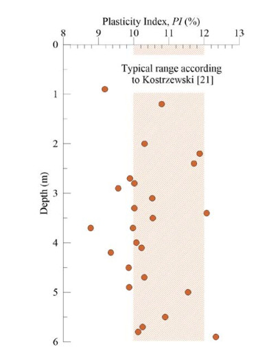
[21]	Kostrzewski W (1988) Parametry geotechniczne gruntów budowlanych oraz metody ich oznaczania (Geotechnical parameters of soil and methods of theirs derivation). Poznań, Poland: Wydawnictwo Politechniki Poznańskiej.
[22]	Młynarek Z, Tschuschke W, Wierzbicki J (1997) Klasyfikacja gruntów podłoża budowlanego metodą statycznego sondowania (Soil classification by means of cone penetration testing), Gdańsk, Poland, 119–127.
[23]	Liszkowski J, Tschuschke M, Młynarek Z, et al. (2004) Statistical evaluation of the dependence of the liquidity index and undrained shear strength of CPTU parameters in cohesive soils. In: Viana da Fonseca A, Mayne PH, editors, 2014, Porto. Millpress, 979–985.
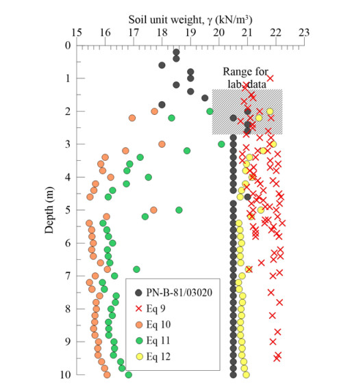
[24]	PKN (1981) PN-81/B-03020; Grunty budowlane. Posadowienie bezpośrednie budowli. Obliczenia statyczne i projektowanie (Polish standard PN/B-03020: Building soils. Foundation bases. Static calculation and design).
[25]	Lasowska A (2018) Analysis of spatial variability of Vistulian glaciation tills unt weight using CPTU probing. Poznań, Poland: Adam Mickiewicz University, 55.
[26]	Robertson PK (2009) Interpretation of cone penetration tests-a unified approach. Can Geotech J 46: 1337–1355. doi: 10.1139/T09-065
[27]	Mayne PW (2014) Interpretation of geotechnical parameters from seismic piezocone tests. In: Robertson PK, Cabal KI, editors, USA: Las Vegas, ISSMGE Technical Committee TC 102, 47–73.
[28]	Marchetti S (1980)In situ tests by flat dilatometer. ASCE Jnl GED 106: 299–321.
[29]	Lunne T, Powel JJM, Hauge EA, et al. (1990) Correlation of Dilatometer Readings to Lateral Stress. Proc of Special Session on Measurement of Lateral Stress, Washington D.C.
[30]	Karlsrud K, Lunne T, Kort DA, et al. (2005) CPTU correlations for clays, Osaka. Millpress, 693–702.
[31]	Kulhawy FH, Mayne PW (1990) Manual on estimating soil properties for foundation design. Electric Power Research Institute, EPRI.
[32]	Młynarek Z, Wierzbicki J, Lunne T (2016) On the influence of overconsolidation effect on the compressibility assessment of subsoil by means of CPTU and DMT. Ann Wars Univ Life Sci Land Reclam 48: 189–200. doi: 10.1515/sggw-2016-0015
[33]	Młynarek Z, Wierzbicki J, Stefaniak K (2013) Deformation characteristics of overconsolidated subsoil from CPTU and SDMT tests. In: Coutinho RQ, Mayne PW, editors, Recife, Taylor & Francis Group, 1189–1193.
[34]	DeJong JT, Jaeger RA, Boulanger RW, et al. (2013) Variable penetration rate cone testing for characterization of intermediate soils. In: Coutinho RQ, Mayne PW, editors, Brazil: Recife, Taylor & Francis Group, 25–42.
[35]	Mayne PW, Peuchen J (2018) Evaluation of CPTU Nkt cone factor for undrained strength of clays. In: Hicks MA, Pisano F, Peuchen J, editors. Cone Penetration Testing 2018, London: Taylor and Francis Group, 423–429.
[36]	Stefaniak K (2015) Assessment of shear strength in silty soils. Stud Geotech Mech 37: 51–55. doi: 10.1515/sgem-2015-0020
[37]	Lechowicz Z, Szymański A (2002) Odkształenia i stateczność nasypów na gruntach organicznych (Deformations and stability of embankments on organic soil), Warszawa, Poland: Wydawnictwo SGGW, 184.

This article has been cited by:

1.	Tariq A. Aljaaidi, Deepak B. Pachpatte, Ram N. Mohapatra, The Hermite–Hadamard–Mercer Type Inequalities via Generalized Proportional Fractional Integral Concerning Another Function, 2022, 2022, 1687-0425, 1, 10.1155/2022/6716830
2.	Saad Ihsan Butt, Ahmet Ocak Akdemir, Muhammad Nadeem, Nabil Mlaiki, İşcan İmdat, Thabet Abdeljawad, $(m, n)$ -Harmonically polynomial convex functions and some Hadamard type inequalities on the co-ordinates, 2021, 6, 2473-6988, 4677, 10.3934/math.2021275
3.	Ifra Bashir Sial, Nichaphat Patanarapeelert, Muhammad Aamir Ali, Hüseyin Budak, Thanin Sitthiwirattham, On Some New Ostrowski–Mercer-Type Inequalities for Differentiable Functions, 2022, 11, 2075-1680, 132, 10.3390/axioms11030132
4.	Deniz Uçar, Inequalities for different type of functions via Caputo fractional derivative, 2022, 7, 2473-6988, 12815, 10.3934/math.2022709
5.	Soubhagya Kumar Sahoo, Y.S. Hamed, Pshtiwan Othman Mohammed, Bibhakar Kodamasingh, Kamsing Nonlaopon, New midpoint type Hermite-Hadamard-Mercer inequalities pertaining to Caputo-Fabrizio fractional operators, 2023, 65, 11100168, 689, 10.1016/j.aej.2022.10.019
6.	Muhammad Imran Asjad, Waqas Ali Faridi, Mohammed M. Al-Shomrani, Abdullahi Yusuf, The generalization of Hermite-Hadamard type Inequality with exp-convexity involving non-singular fractional operator, 2022, 7, 2473-6988, 7040, 10.3934/math.2022392
7.	Churong Chen, Discrete Caputo Delta Fractional Economic Cobweb Models, 2023, 22, 1575-5460, 10.1007/s12346-022-00708-5
8.	Soubhagya Kumar Sahoo, Ravi P. Agarwal, Pshtiwan Othman Mohammed, Bibhakar Kodamasingh, Kamsing Nonlaopon, Khadijah M. Abualnaja, Hadamard–Mercer, Dragomir–Agarwal–Mercer, and Pachpatte–Mercer Type Fractional Inclusions for Convex Functions with an Exponential Kernel and Their Applications, 2022, 14, 2073-8994, 836, 10.3390/sym14040836
9.	Muhammad Tariq, Sotiris K. Ntouyas, Asif Ali Shaikh, A Comprehensive Review of the Hermite–Hadamard Inequality Pertaining to Fractional Integral Operators, 2023, 11, 2227-7390, 1953, 10.3390/math11081953
10.	Loredana Ciurdariu, Eugenia Grecu, Hermite–Hadamard–Mercer-Type Inequalities for Three-Times Differentiable Functions, 2024, 13, 2075-1680, 413, 10.3390/axioms13060413
11.	Muhammad Aamir Ali, Thanin Sitthiwirattham, Elisabeth Köbis, Asma Hanif, Hermite–Hadamard–Mercer Inequalities Associated with Twice-Differentiable Functions with Applications, 2024, 13, 2075-1680, 114, 10.3390/axioms13020114
12.	Muhammad Aamir Ali, Christopher S. Goodrich, On some new inequalities of Hermite–Hadamard–Mercer midpoint and trapezoidal type in q-calculus, 2024, 44, 0174-4747, 35, 10.1515/anly-2023-0019
13.	Thanin Sitthiwirattham, Ifra Sial, Muhammad Ali, Hüseyin Budak, Jiraporn Reunsumrit, A new variant of Jensen inclusion and Hermite-Hadamard type inclusions for interval-valued functions, 2023, 37, 0354-5180, 5553, 10.2298/FIL2317553S
14.	Muhammad Aamir Ali, Zhiyue Zhang, Michal Fečkan, GENERALIZATION OF HERMITE–HADAMARD–MERCER AND TRAPEZOID FORMULA TYPE INEQUALITIES INVOLVING THE BETA FUNCTION, 2024, 54, 0035-7596, 10.1216/rmj.2024.54.331
15.	Bahtiyar Bayraktar, Péter Kórus, Juan Eduardo Nápoles Valdés, Some New Jensen–Mercer Type Integral Inequalities via Fractional Operators, 2023, 12, 2075-1680, 517, 10.3390/axioms12060517
16.	THANIN SITTHIWIRATTHAM, MIGUEL VIVAS-CORTEZ, MUHAMMAD AAMIR ALI, HÜSEYIN BUDAK, İBRAHIM AVCI, A STUDY OF FRACTIONAL HERMITE–HADAMARD–MERCER INEQUALITIES FOR DIFFERENTIABLE FUNCTIONS, 2024, 32, 0218-348X, 10.1142/S0218348X24400164
17.	Muhammad Ali, Hüseyin Budak, Elisabeth Köbis, Some new and general versions of q-Hermite-Hadamard-Mercer inequalities, 2023, 37, 0354-5180, 4531, 10.2298/FIL2314531A

Reader Comments

Your name:*

Email:*
© 2019 the Author(s), licensee AIMS Press. This is an open access article distributed under the terms of the Creative Commons Attribution License (http://creativecommons.org/licenses/by/4.0)